Understanding Transformers: The Mathematical Foundations of Large Language Models

In recent years, two major breakthroughs have revolutionized the field of Large Language Models (LLMs):

1. 2017: The publication of Google’s seminal paper, (https://arxiv.org/abs/1706.03762) by Vaswani et al., which introduced the Transformer architecture – a neural network that fundamentally changed Natural Language Processing (NLP).
2. 2022: The launch of ChatGPT by OpenAI, a transformer-based chatbot that demonstrated the power of Generative Pre-trained Transformers (GPT) in real-world applications.

This blog post will dive deep into the mathematical foundations of the Transformer architecture, explaining its core mechanisms—self-attention, multi-head attention, and positional encoding – with detailed derivations and illustrations.

1. Language Models: Discriminative vs. Generative Tasks

Language models are trained to perform various tasks, such as:

– Discriminative tasks (e.g., sentiment analysis, text classification)
– Generative tasks (e.g., question answering, code generation, text completion)

A key challenge in NLP is understanding context – how words relate to each other, even when far apart. For example:

> “The woman is the sole survivor, and wanders off in a daze; she hides in an apartment when the occupant leaves with suitcases.”

Here, “she” refers to “the woman”, and “leaves” refers to the “apartment”. Traditional models like CNNs struggle with such long-range dependencies because they rely on local receptive fields.

Why Transformers?
– CNNs assume that the most relevant information is in neighboring pixels (or tokens).
– RNNs/LSTMs process sequences sequentially, making them slow and prone to forgetting early tokens.
– Transformers use self-attention, allowing them to weigh the importance of all tokens simultaneously.

2. The Transformer Architecture: Core Components

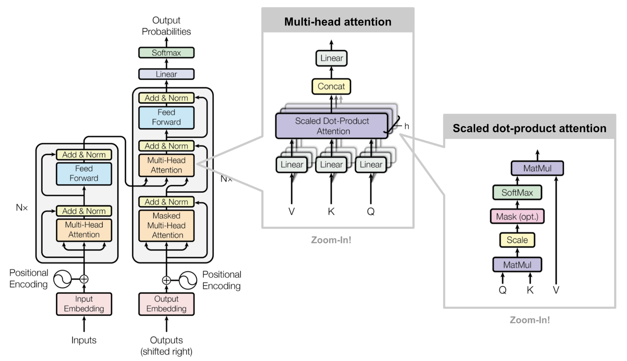
The Transformer consists of:
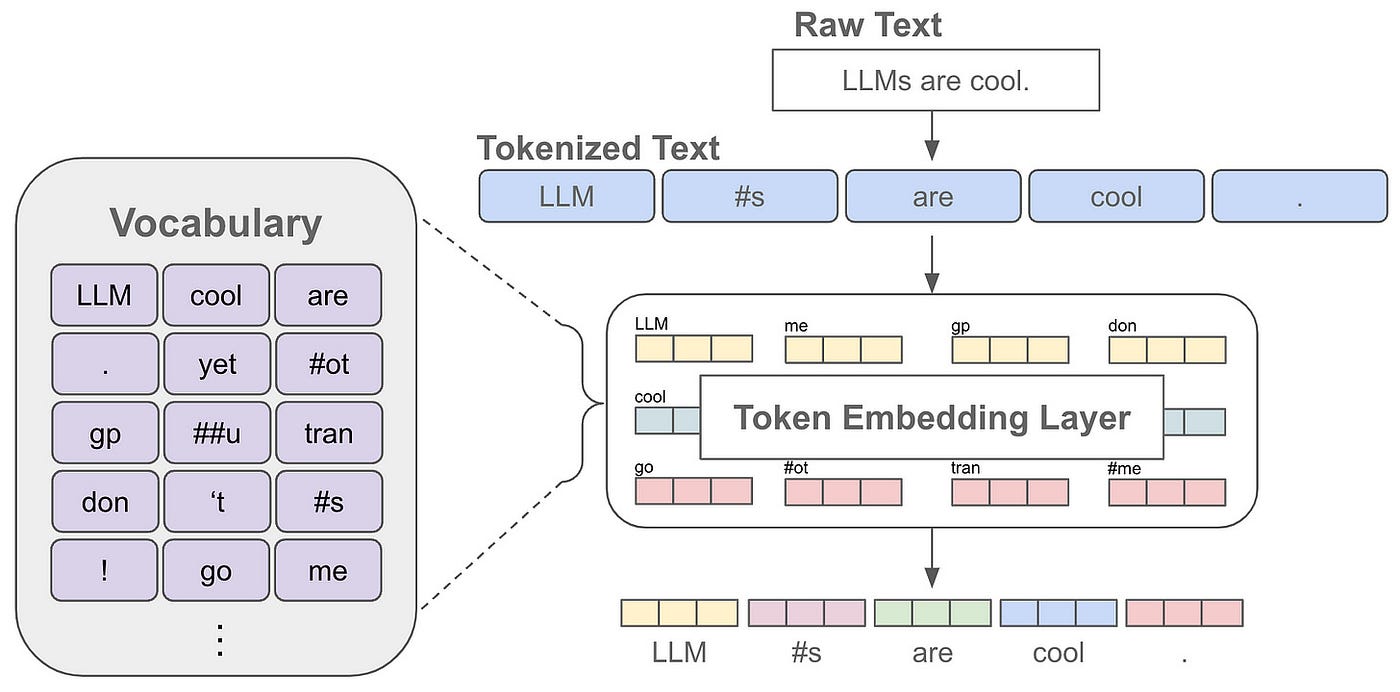
1. Token Embeddings (converting words into vectors)
2. Positional Encoding (adding positional information)
3. Self-Attention Mechanism (computing token relationships)
4. Feed-Forward Networks (non-linear transformations)
5. Layer Normalization & Residual Connections (stabilizing training)

We will focus on the self-attention mechanism, the heart of the Transformer.

3. Self-Attention: Mathematical Formulation

Step 1: Input Representation
Each token is represented as a vector \( \mathbf{x}_i \in \mathbb{R}^d \), where \( d \) is the embedding dimension.

Step 2: Query, Key, and Value Matrices
The Transformer learns three weight matrices:
– \( \mathbf{W}^Q \in \mathbb{R}^{d \times d_k} \) (Query)
– \( \mathbf{W}^K \in \mathbb{R}^{d \times d_k} \) (Key)
– \( \mathbf{W}^V \in \mathbb{R}^{d \times d_v} \) (Value)

For each token \( \mathbf{x}_i \), we compute:
\[
\mathbf{q}_i = \mathbf{x}_i \mathbf{W}^Q \quad \text{(Query)}
\]
\[
\mathbf{k}_i = \mathbf{x}_i \mathbf{W}^K \quad \text{(Key)}
\]
\[
\mathbf{v}_i = \mathbf{x}_i \mathbf{W}^V \quad \text{(Value)}
\]

Step 3: Attention Scores
The attention score between token \( i \) and token \( j \) is computed using the dot product:
\[
a_{ij} = \frac{\mathbf{q}_i \mathbf{k}_j^T}{\sqrt{d_k}}
\]
where \( \sqrt{d_k} \) is a scaling factor to prevent large gradients.

Step 4: Softmax Normalization
The scores are normalized using softmax to obtain attention weights:
\[
\alpha_{ij} = \text{softmax}(a_{ij}) = \frac{\exp(a_{ij})}{\sum_{l=1}^n \exp(a_{il})}
\]

Step 5: Weighted Sum of Values
The final output for token \( i \) is a weighted sum of all value vectors:
\[
\mathbf{z}_i = \sum_{j=1}^n \alpha_{ij} \mathbf{v}_j
\]

Step 6: Multi-Head Attention
Instead of a single attention head, Transformers use multiple heads (e.g., 8 in the original paper). Each head has its own \( \mathbf{W}^Q, \mathbf{W}^K, \mathbf{W}^V \), allowing the model to capture different relationships.

The outputs of all heads are concatenated and linearly transformed:
\[
\mathbf{Z} = \text{Concat}(\mathbf{z}_1, \mathbf{z}_2, \dots, \mathbf{z}_h) \mathbf{W}^O
\]
where \( \mathbf{W}^O \in \mathbb{R}^{h d_v \times d} \).

Step 7: Residual Connection & Layer Normalization
To stabilize training, the output is added to the original input and normalized:
\[
\mathbf{Z}_{\text{out}} = \text{LayerNorm}(\mathbf{Z} + \mathbf{X})
\]

4. Positional Encoding

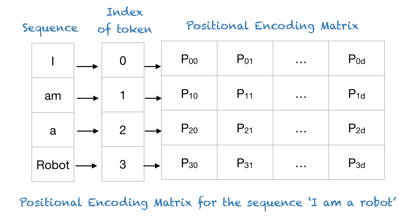
Since Transformers process tokens in parallel (unlike RNNs), they need a way to encode positional information. This is done using sinusoidal functions:
\[
PE_{(pos, 2i)} = \sin\left(\frac{pos}{10000^{2i/d}}\right)
\]
\[
PE_{(pos, 2i+1)} = \cos\left(\frac{pos}{10000^{2i/d}}\right)
\]
where:
– \( pos \) = token position
– \( i \) = dimension index

This ensures that relative positions are captured in a way that generalizes to longer sequences.

5. Feed-Forward Network (FFN)

After self-attention, each token passes through a two-layer FFN:
\[
\text{FFN}(\mathbf{z}) = \text{ReLU}(\mathbf{z} \mathbf{W}_1 + \mathbf{b}_1) \mathbf{W}_2 + \mathbf{b}_2
\]
where \( \mathbf{W}_1 \in \mathbb{R}^{d \times d_{ff}} \), \( \mathbf{W}_2 \in \mathbb{R}^{d_{ff} \times d} \).

6. Training & Next-Token Prediction

To train a generative model (like GPT), the objective is to predict the next token given previous tokens:
\[
P(x_t | x_{<t}) = \text{softmax}(\mathbf{W} \mathbf{z}_t + \mathbf{b})
\]
where:
– \( \mathbf{z}_t \) = final hidden state at position \( t \)
– \( \mathbf{W} \in \mathbb{R}^{|V| \times d} \) (vocabulary projection)
– \( \mathbf{b} \in \mathbb{R}^{|V|} \) (bias)

The model is trained using cross-entropy loss:
\[
\mathcal{L} = -\sum_{t=1}^T \log P(x_t | x_{<t})
\]

7. Summary & Key Takeaways
1. Self-Attention allows the model to weigh the importance of all tokens simultaneously.
2. Multi-Head Attention captures different types of relationships (e.g., syntactic, semantic).
3. Positional Encoding ensures the model understands token order.
4. Residual Connections & LayerNorm stabilize deep networks.
5. Next-Token Prediction is optimized via cross-entropy loss.

Why Transformers Dominate NLP
– Parallel processing (faster than RNNs)
– Long-range dependencies (better than CNNs)
– Scalability (works well with large datasets)

Final Thoughts
The Transformer architecture is a breakthrough in deep learning, enabling models like GPT-4, BERT, and T5. Understanding its mathematical foundations helps in designing better models and debugging training issues.

Would you like a deeper dive into optimization techniques (e.g., AdamW, learning rate scheduling) or efficiency improvements (e.g., sparse attention, mixture-of-experts)? Let me know in the comments!

References
1. Vaswani et al. (2017). (https://arxiv.org/abs/1706.03762).
2. OpenAI. (2022). (https://openai.com/blog/chatgpt/).
3. Jay Alammar. (https://jalammar.github.io/illustrated-transformer/).