Convolutional Neural Networks (CNNs) have become the cornerstone of image and video recognition in the world of deep learning. From self-driving cars to medical image analysis, CNNs are everywhere, powering applications that rely on understanding visual data. But how do CNNs actually work? What are their components, and how do they process images to make sense of complex patterns? In this blog post, we’ll explore the fundamentals of CNNs, breaking down their components, working principles, and how they’re used in real-world applications.

What Is a Neural Network?

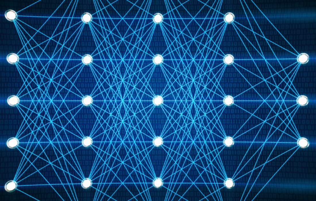
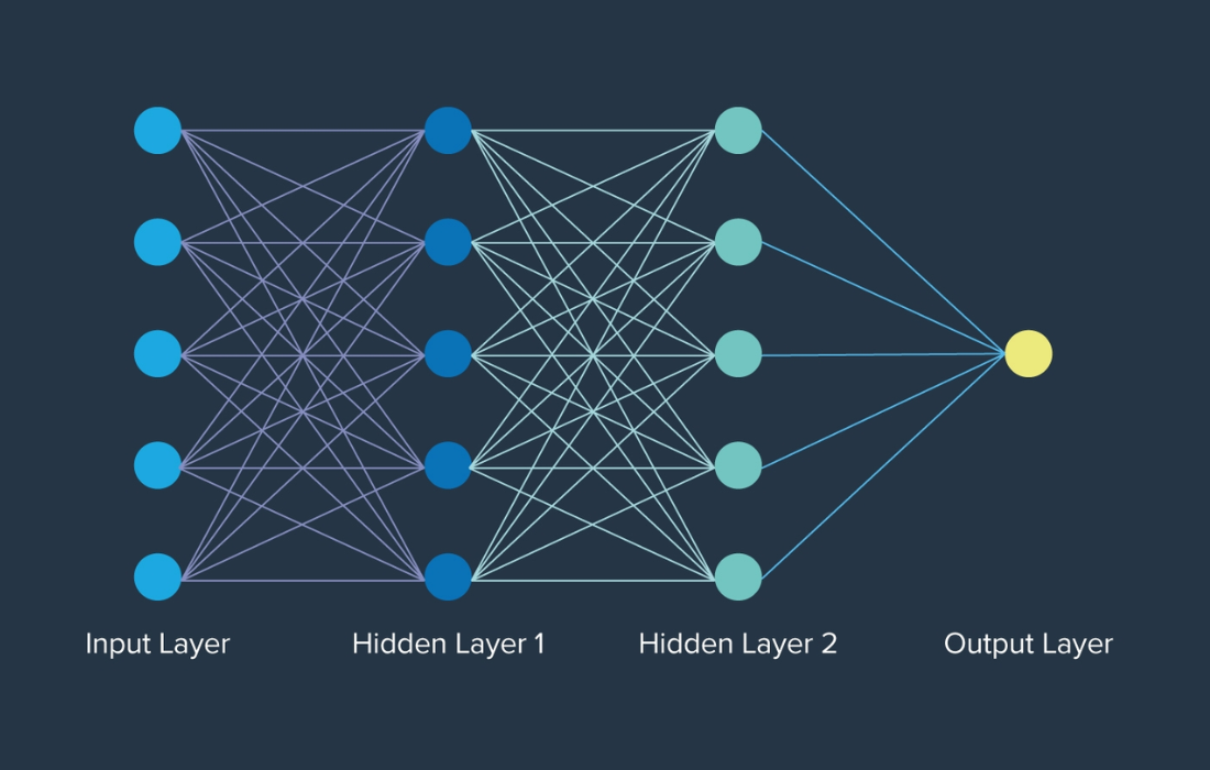
Before diving into CNNs, let’s take a moment to understand what a neural network is. At its core, a neural network is an artificial system designed to mimic the workings of the human brain. It consists of layers of nodes (or “neurons”) connected in a web-like structure, where each node performs a mathematical operation. The strength of the connection between the nodes (called weights) is learned through training, allowing the network to make intelligent decisions or predictions.

What Is a Convolutional Neural Network (CNN)?

A Convolutional Neural Network is a specialized type of neural network that excels in processing grid-like data, particularly images and videos. It’s designed to automatically and adaptively learn patterns and features in images, making it much more efficient than traditional machine learning algorithms for visual data. CNNs perform tasks such as image classification, face recognition, object detection, and medical image analysis.

The key difference between a CNN and a traditional Artificial Neural Network (ANN) is that CNNs have built-in mechanisms, such as convolution and pooling, to handle image data efficiently. Instead of relying on raw pixel values as input, CNNs can extract features from the image automatically, reducing the need for extensive manual feature engineering.

Understanding Convolution in CNNs

At the heart of a CNN is the “convolution” operation, which is a mathematical process that combines two matrices to produce a new one. When applied to images, the convolution operation helps to detect patterns, such as edges, textures, or shapes. This is what makes CNNs particularly effective in image-related tasks.

The process begins with an image (represented as a matrix of pixel values) and a small filter (or kernel) that slides over the image. The filter performs an element-wise multiplication with the image matrix, followed by summing the results. This is repeated as the filter slides across the entire image, generating a “feature map” that highlights the patterns detected by the filter.

Image Representation in CNNs

Before we get into the layers of a CNN, it’s important to understand how images are represented in a way that the model can process. Images are essentially grids of pixels, and each pixel has a value that represents its color or intensity.

There are two common types of images:

1. Grayscale Images: These images have only one channel, representing the intensity of light, with pixel values ranging from 0 (black) to 255 (white).
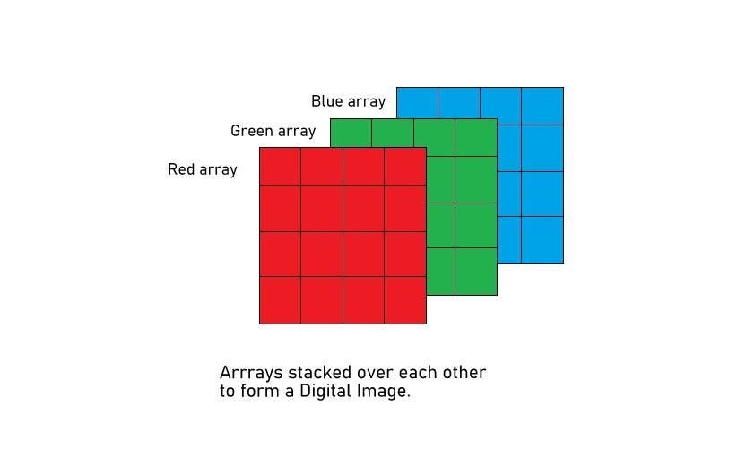
2. RGB Images: These images have three channels, representing red, green, and blue colors. Each pixel has three values, one for each channel, which together form a full-color image.

Components of a CNN

A typical Convolutional Neural Network consists of the following key layers:

1. Convolution Layer
2. Pooling Layer
3. Fully Connected Layer

Let’s take a closer look at each of these layers.

1. Convolution Layer

The convolution layer is where the actual “convolution” operation takes place. Here, filters (also known as kernels) are applied to the input image to detect specific patterns, such as edges, corners, or textures. These filters are small matrices that “slide” over the image, performing element-wise multiplication with the image data, and then summing the results to form a feature map.

The feature map reveals where specific features, like edges or textures, are located in the image. Filters are learned during the training process using backpropagation, which helps the model to adjust the filters to detect relevant patterns for the task at hand.

2. Pooling Layer

After the convolution layer, we apply a pooling layer to reduce the spatial dimensions of the feature map while retaining important features. Pooling is essentially a down-sampling operation that helps reduce computational complexity and prevents overfitting.

There are two types of pooling:

• Max Pooling: This takes the maximum value from a specific region of the feature map.
• Average Pooling: This computes the average value of the region.

By reducing the size of the feature maps, pooling allows the model to focus on the most important features while discarding less relevant details.

3. Fully Connected Layer

Once the image has passed through multiple convolution and pooling layers, it’s time for the final stage—flattening. The pooled feature maps are converted into a one-dimensional array, which is then fed into a fully connected layer. This layer works like a traditional artificial neural network, where each neuron is connected to every neuron in the previous layer. The fully connected layer performs classification or regression tasks based on the features extracted by the previous layers.

Key Techniques: Padding and Striding

There are two important techniques used in CNNs to control the size of the feature maps and improve the model’s performance:

1. Padding: Padding involves adding zero-value pixels around the border of the image before applying the convolution operation. This helps to ensure that features at the edges of the image are not ignored and are properly incorporated into the feature map.
2. Striding: Striding refers to how much the filter shifts over the image after each convolution operation. By adjusting the stride, we can control the size of the feature map and make the model more efficient.

How Does CNN Work for Image Classification?

Now that we’ve covered the basics of CNNs, let’s discuss how they can be used for image classification. Suppose we want to classify images of animals (e.g., cats, dogs, etc.). The CNN will process the image through multiple layers—starting with convolution and pooling to detect low-level features (like edges or textures) and moving up to higher-level features (like shapes or patterns).

As the image passes through each layer, the model extracts increasingly complex features. By the time the image reaches the fully connected layer, the model has learned to recognize enough features to classify the image correctly.

Real-World Applications of CNNs

CNNs have revolutionized several fields, thanks to their ability to automatically detect patterns in visual data. Some of the key applications include:

• Object Detection: Detecting and localizing objects within images or videos.
• Facial Recognition: Identifying or verifying individuals based on facial features.
• Medical Imaging: Analyzing medical scans (e.g., MRIs, X-rays) to detect diseases or abnormalities.
• Self-Driving Cars: Enabling autonomous vehicles to understand and navigate their environment.

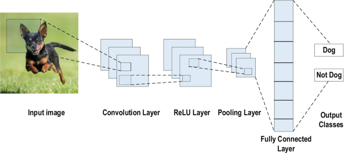
We just put an image into CNN, it figures it automatically how to deal with it. How convenient is it? No boring preprocessing, No OpenCV. I mean there is a valid reason why CNNs have so many real-world applications, from Self-driving cars to Medical imaging, it is used everywhere!

Ok, so now we know that CNN is good at handling Image-related data, but how does CNN do this? Let’s find out!

But before understanding how CNN works let’s understand how Images are represented digitally.

Images and their representation

To put it simply, An Image is a large square divided into several sub-squares, each subsquare is called a Pixel. Pixels are the basic building blocks of the image.

Every pixel has an assigned pixel value (or set of values). These pixel values describe the intensity and color at that point. The subtle combination of these pixels in a structured manner is what makes an image unique.

Now, there are two types of images: 1. Grayscale 2. RGB. These are nothing but fancy scientific terms for a Black and white image and a colored image.

For a grayscale image, Each pixel in a grayscale image is represented by a single value that denotes its brightness or intensity. The value typically ranges from 0 (black) to 255 (white) in an 8-bit grayscale image. Grayscale images have only one channel, representing the intensity of light. It’s like looking at the world through a single lens that captures only the brightness.

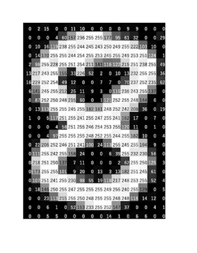
RGB images are full-color images that include red, green, and blue color channels. Each pixel in an RGB image is represented by three values, one for each color channel (red, green, and blue). Each of these values can range from 0 to 255, determining the intensity of that color in the pixel. RGB images have three channels, and when combined, these channels create a wide spectrum of colors. It’s like having three lenses (red, green, and blue) that capture different aspects of the scene. Combinations of pixel values at Red, Blue, and Green channels form a Coloured image.

Components of CNN

On a bigger picture, a CNN has three layers:

1. Convolution Layer
2. Pooling Layer
3. Fully Connected Layer

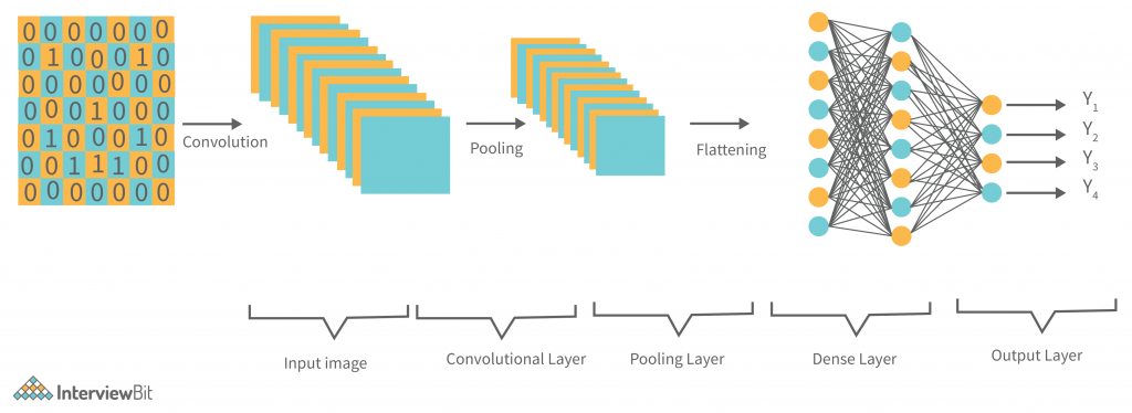
The above 2 layers — The convolution layer and the Pooling layer are what make CNNs different from ANNs. It’s the combination of the first two layers with ANN, ie. the Fully Connected Layer.

Let’s study each of them one by one in detail.

Convolution Layer

In this layer, that special ‘Convolution’ operation takes place. (Well, duh!)

But what is Convolution and How it works?

Suppose we have two matrices M1 and M2. And let’s say the convolution of M1 and M2 produces an output matrix M3. ie:

M1 * M2 = M3

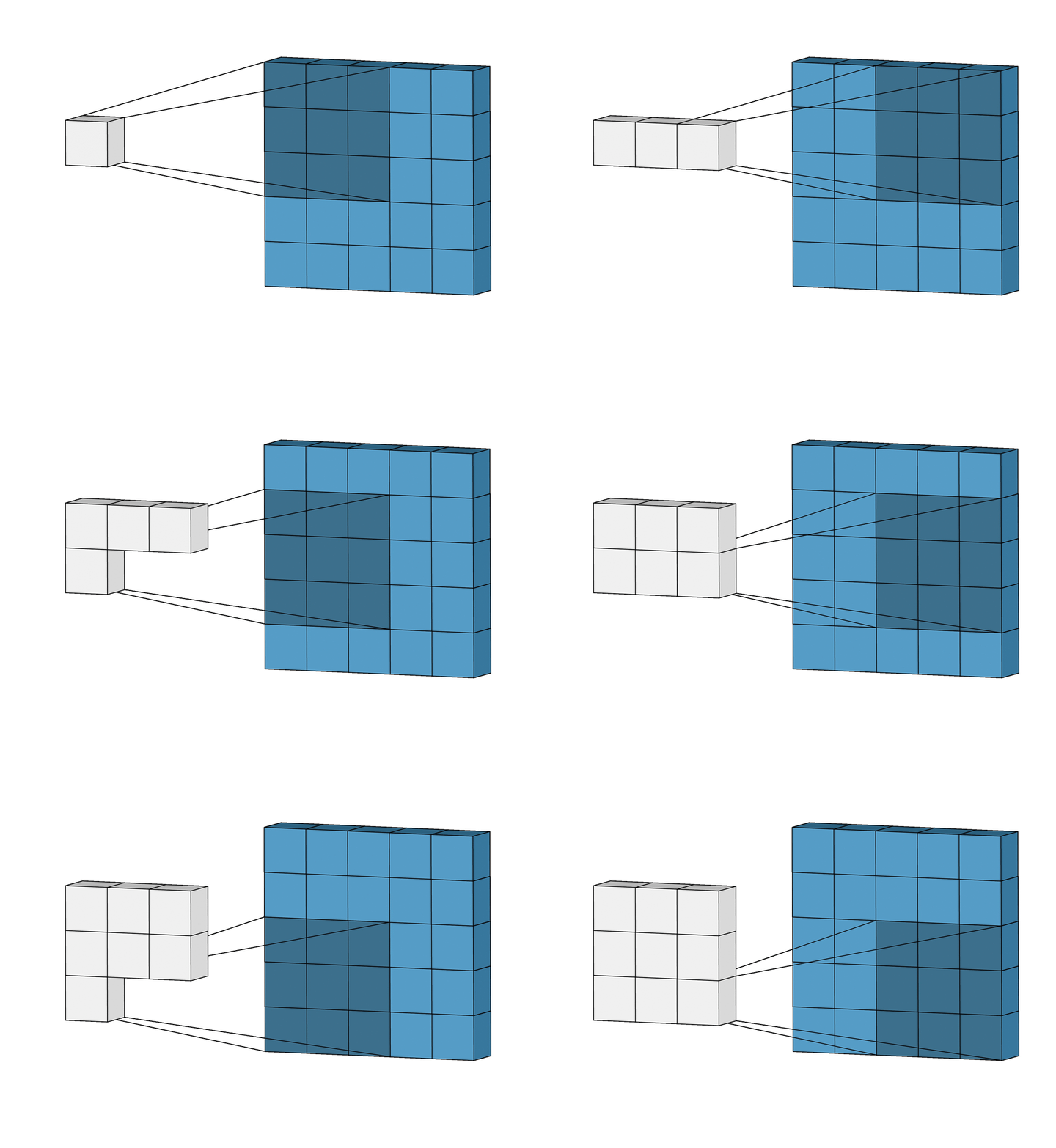
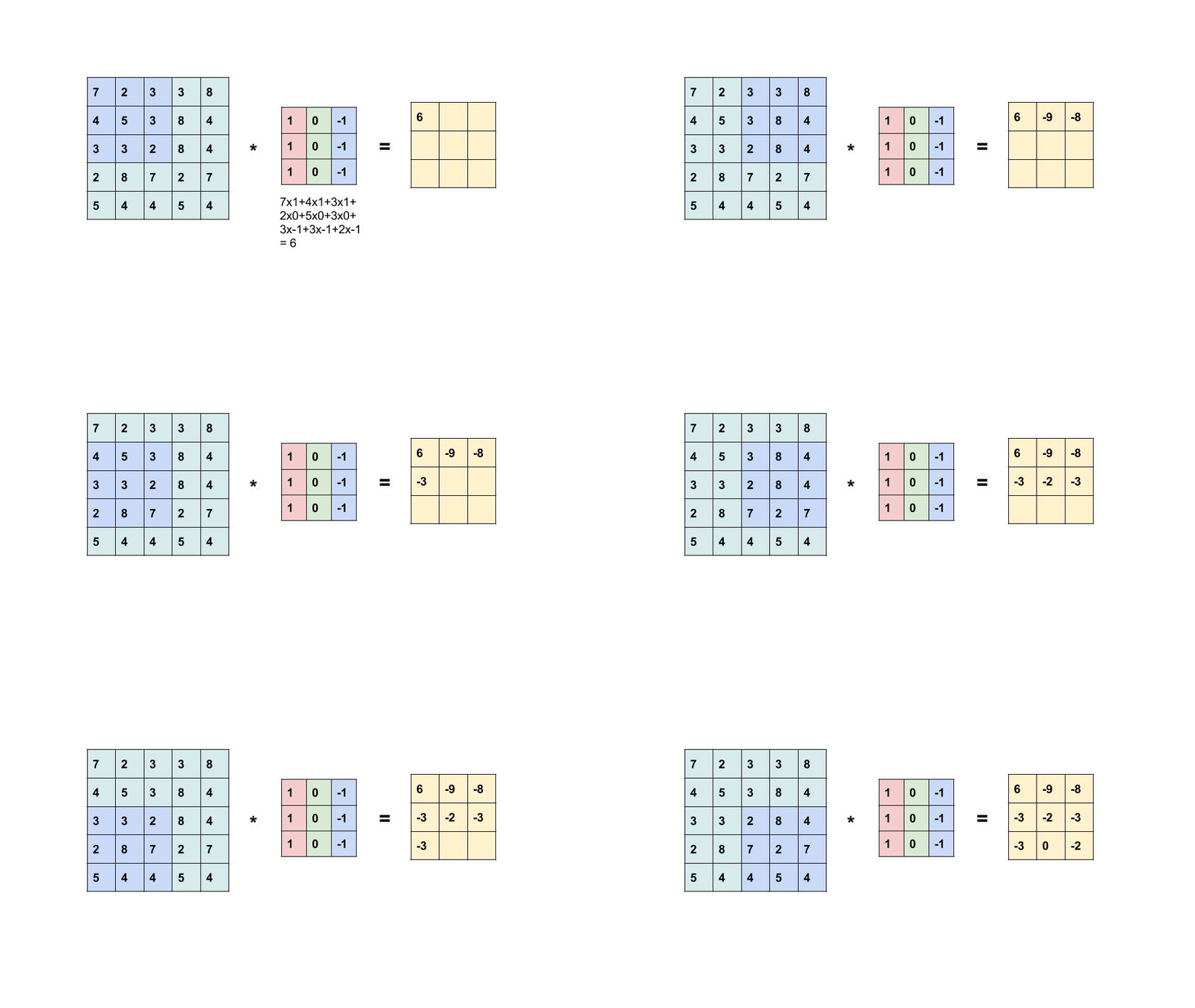
So, to calculate M1 * M2 (Convolution of M1 and M2), we place M2 over the top left corner of M1, do element-wise multiplication of those elements that M2 covers at M1, and sum these products. This alone would be the one element of M3. Then we shift M2 by 1 column and do the same thing. This would be the next element of M3. In this way, all the elements of M3 are calculated. This is the essence of Convolution in the context of matrices.

Now, why are we talking about matrices? Remember, we talked about the representation of images in the above section? Yes, an image (grayscale) is a matrix of pixel values. So, it acts as M1. What about M2? We use a special type of matrix called ‘Filter’ over images, these act as M2. The convolution of Image (I) with a filter (F) results in the formation of Feature Map (M), which acts as M3.

So, just like the above general example, a filter will be placed over the top left corner of the image, perform element-wise products of coincided elements and then these are summed. Then, the filter will get shifted by one pixel, and do the same thing over the image, to produce a third type of matrix called a Feature Map.

So: I * F = M (Image * Filter = Feature Map)

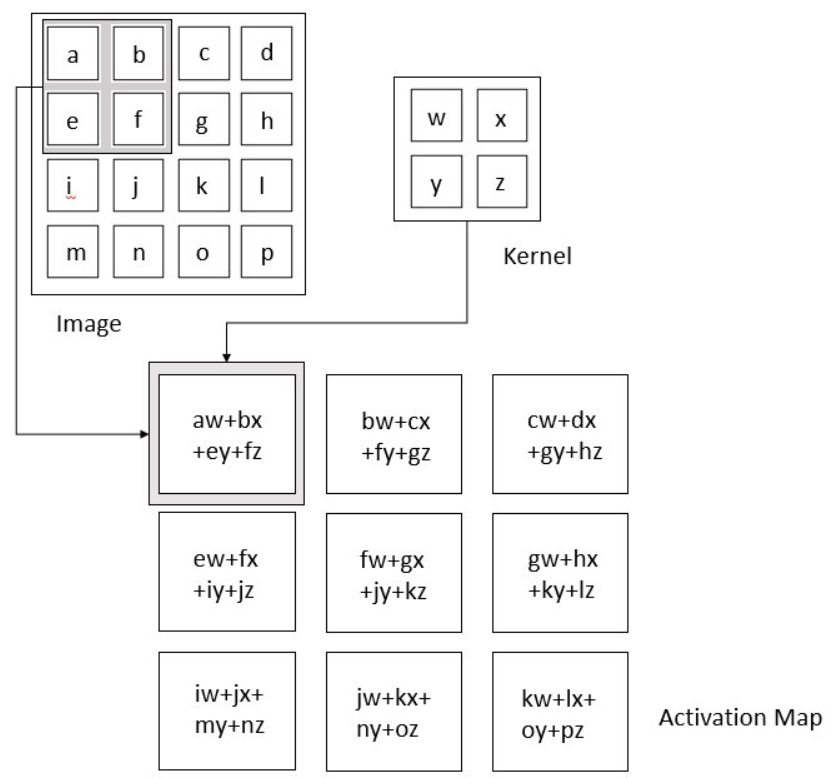
Wait, I get it, so much to take in. First of all, what are filters? Well, Filters (or kernels) act as ‘feature detectors’. These are used to find certain patterns or shapes in an image. These filters can be of different types. Some types of filters are used to find only edges, while others are used to find any corners or other complex patterns in the image.

By the way, these filters are just some special matrices with fixed numerical pixel values as their elements.

When these filters are convolved over an image, a feature map is produced, which tells the presence of these features or patterns in these images. These feature maps are the outputs of the convolution layer, while acting as inputs for the next layer.

In layman’s terms, a filter is used to find patterns in the image while feature maps tell where these patterns are in the image.

Note: Multiple Filters or kernels are going to be used to capture every kind of pattern in the image. There are different kinds of filters to identify different kinds of patterns in images.

These patterns we are talking about are nothing but subtle combinations and arrangements of pixels in there image.

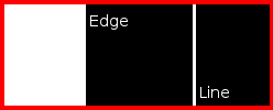
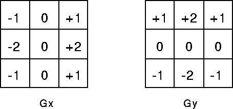
For example, to detect different types of edges in the image, we use a specific kind of filter called ‘The Sobel Filter’. Similarly, other kinds of filters exist to detect other kinds of patterns.

I won’t go into the details of it, to study this, refer to this article:

https://kharshit.github.io/blog/2018/12/14/filters-in-convolutional-neural-networks

To study more deeply about the types of filters used, kindly refer to this amazing article: https://iq.opengenus.org/convolution-filters/

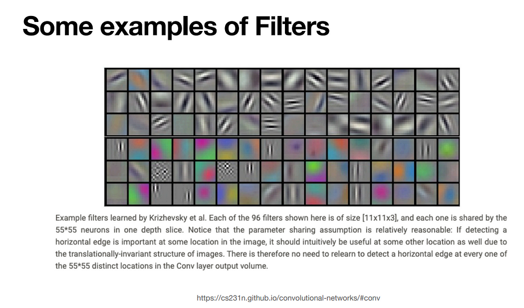
Note: In convolutional neural networks, the filters are learned the same way as hyperparameters through backpropagation during the training process.

Okay, so now we know the fundamentals of Convolution. But this is not the end. To make the model capture complex patterns and features, we need to pass the feature map to an activation function. The most common (in fact, the only) activation function used in the convolution layer is ReLU. Rectified Linear Unit, is an activation function used to capture complex patterns in any type of problem, hence trendy in various Neural network architectures. Mathematically it is defined as:

def ReLU(x):
if x >= 0:
 return x
else:
 return 0

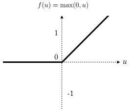
To study more about ReLU and other activation functions, kindly refer to this article:

https://www.analyticsvidhya.com/blog/2020/01/fundamentals-deep-learning-activation-functions-when-to-use-them/

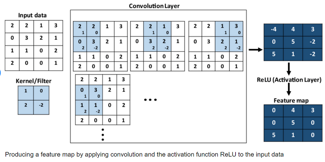
In the case of RGB images, everything is the same just the dimensions are more. Instead of talking in terms of matrices, we talk with tensors.

Alright now, we studied different components of the convolution layer. Before jumping into the next layer, we shall also discuss about two important concepts: 1. Padding 2. Striding. These ‘techniques’ can be used to generate more accurate feature maps during the convolution process. Let’s study them in detail.

Padding

Are you familiar with Padding in CSS? If yes, that’s pretty much what Padding is in the context of Convolutional Neural Networks. Padding, in layman’s terms, is adding ‘zero-valued’ pixels on all four sides of the image, then performing convolution operation over THERE. By this, the features at the edges of the images are more involved and thus are more considered in the feature map. In traditional convolution, the pixels at the borders are less involved in the convolution, thus less prevalent in the feature map, padding solves this problem.

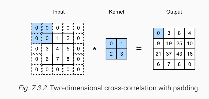
You have noticed that in traditional convolution, the dimension of the feature map is less than that of the dimension of the image. Now in a practical scenario, we apply multiple convolution layers. Like, if an image is passed through multiple convolution layers, the size of the final feature map will be much smaller. So, to deal with this problem, padding is applied when the filter or kernel is convolved over the image. Thus, the size of the feature map produced is not reduced and the important patterns from the image are not missed. Padding helps control the dimension of the feature map and thus, helps preserve important features and patterns in the image during convolution.

Generally, one layer of padding on the image is enough for most of the problems. Two or more layers of padding on the image borders are rarely used (or not used at all) for any problem

Nice, so we discussed about padding. Let’s also discuss another important technique like padding which is used to control the dimension of the feature map: Striding

Striding

It decides, by how many units the filter (or kernel) will shift over the image after computing the first set of dot products (element-wise products). In traditional convolutions, it is set to 1. But we can set it to other values and based on that dimensions of the feature map is controlled.

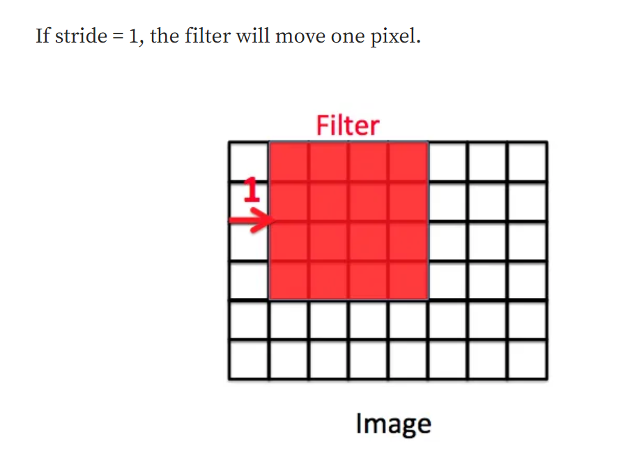
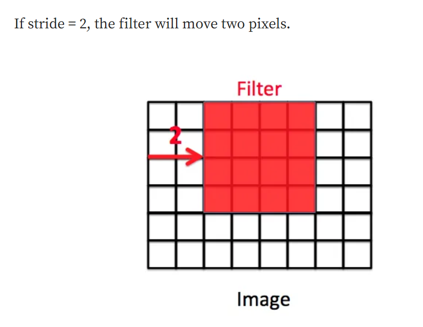
See, it’s as simple as that. However, the default value is still considered for most of the architectures. As we increase striding, the dimension of the feature map keeps getting reduced. For higher values of striding, the filters will miss some pixels while convolving over the image, thus size reduction and potentially missing some important patterns from the image. So, either a proper tradeoff between padding value and stride value is considered or the default is taken (the latter case gives better results, empirically speaking).

Let’s see how the dimensions of the feature map are controlled by padding and striding mathematically in convolution operation:

Here,

n = > Dimension of image. (n x n)

f => Dimension of filter (f x f)

p => Padding value (or the number of layers in padding, default = 0)

s => Striding value (default = 1)

Here,

n => Dimension of image (n x n)

f => Dimension of the filter (or kernel, f x f)

Great, now you are all well versed with how the convolution layer works in a proper sense. Now let’s jump into the next layer in a general CNN architecture, which is…

The Pooling Layer

Well, the bookish definition is:

“ Pooling is a down-sampling operation commonly used in convolutional neural networks (CNNs) to reduce the spatial dimensions of the input data while retaining important features. ”

I know, this definition went over your head….

To put this into simple words, Pooling is the technique for gaining the most important and useful features from the convolved feature map.

The Pooling operation is somewhat similar to how filters are involved in convolution. Here, the ‘Pooling’ filter (with a stride value of 2 and filter size of 2×2) interacts with the feature map and produces the ‘Pooled’ feature map. But what is this operation and how this operation is taking place?

After the image is passed through the convolution layer, a feature map is formed. Now, this special ‘Pooling’ filter (window would be a better word) is placed over the top left corner of the feature map. The pixel values of the feature map that are inside this filter are considered to form the first-pixel value of the ‘Pooled’ feature map. This ‘consideration’ depends upon the type of Pooling we are using.

If we use Max Pooling, the max pixel value inside that filter is taken as the pixel value for the pooled output feature map. If we are using Average Pooling, then the average of the pixel values inside that pooling window becomes the pixel value for the Pooled feature map. After this, the pooling window shifts by 2 pixels and the process repeats over the new set of pixel values inside that window. Thus, the pooled feature map is formed.

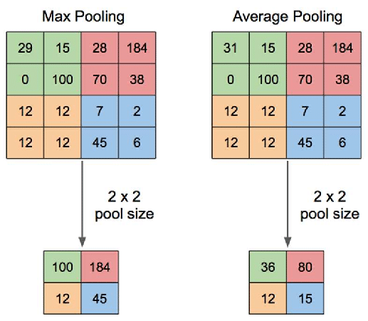
This also makes sense. By applying Pooling, we are Pooling out (or extracting) the most standout pixels or an average of the pixels (or patterns) from the feature map, thus it’s aptly named ‘Pooling’ Lol!

One thing to note here is that in Pooling, the Pooling filter is essentially a window and not a matrix containing pixel values. Instead of an element-wise product, it is the means of gathering the most useful pixels from that specific cluster of pixels inside that window, thereby eliminating useless pixels and features.

Another important advantage of the Pooling operation is that it is ‘Translation Invariant’. I know, a very fancy term, let me explain.

Suppose, You have an image of a Cat. So no matter how the cat is positioned in the image. It can be upside down, it can be of small size, slightly tilted, or not aligned at the center, it is still an image of a cat, right? YES. This is what Translational invariance is in the context of images. We can identify through the image that its a cat but how CNN can do it? Well, though Pooling. Thus, it’s an essential layer in CNN.

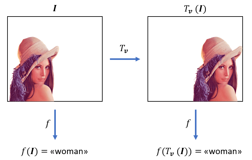
So, the main point? Some variations in the image should not hinder classification ability. Thus the term ‘invariance’. This property of CNN helps it to generalize better.

Alright, the Convolution layer is done. The pooling layer. done. Now what?

Flattening

After the pooling operation, the feature map is converted into a Pooled feature map. But it is still a matrix (or tensor in the case of RGB images), it is NOT one-dimensional. As we discussed at the beginning that image is first converted in such a form that can act as an input for ANN. But, we cannot put this pooled feature map into the ANN. We first have to make it a one-dimensional format. How do we do this? Through Flattening layer! I mean it was obvious by the name, that we ‘Flatten’ the pooled feature map in the form of one one-dimensional array.

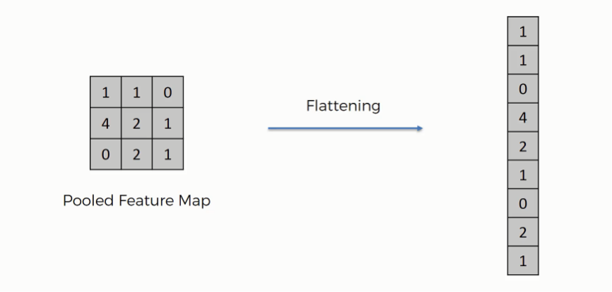
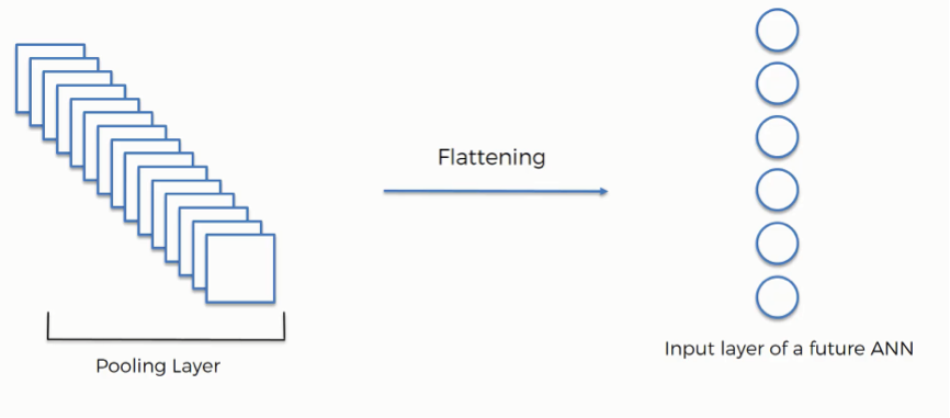
Mathematically also, it is not rocket science. it is just re-arranging all the elements of the pooled feature map linearly. THATS IT!

Now, this flattened array is ready to be put into the ANN or we call it…

Fully Connected Layer

That’s it we are almost there. We studied the difficult portion. In the above sections, we studied the part of CNN that separates it from an ANN.

This layer, the Fully Connected layer as we call is just a typical artificial neural network.

So, the flattened array we generated in the last layer acts as the numerical input for the Fully Connected layer. And, that’s it, from here on onwards the work will be similar to how an ANN responds to numerical inputs. . Yes, those same interconnections of neurons with weights and biases involved blah blah and all that backpropagation stuff. I won’t go into much detail otherwise the article will be too long (It is already very long).

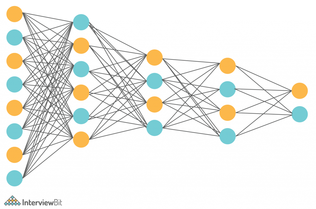
Note: These are the basic building blocks of CNN. We can have so many variations by tweaking the numbers or number of layers involved and BOOM! A new CNN architecture is born. So many architectures of CNN like LeNet, AlexNet, VGGNet, Inception, etc are formed just by tweaking these building blocks and numbers. In this article, however, we only focused on the basic building blocks, working, and intuition behind CNN.

Conclusion

Convolutional Neural Networks (CNNs) are a powerful tool for image processing, capable of automatically extracting and learning complex patterns from images. By using convolution and pooling layers to process images, CNNs can efficiently handle large amounts of visual data. Whether you’re dealing with medical images, satellite data, or facial recognition, CNNs are the go-to choice for solving image-related problems. As deep learning continues to evolve, CNNs will remain a foundational technology for a wide range of applications.

References

https://www.upgrad.com/blog/basic-cnn-architecture/