Neural networks are the backbone of modern artificial intelligence (AI), powering applications like image recognition, natural language processing, and autonomous vehicles. However, behind their impressive capabilities lies a deep mathematical framework that makes them effective. This blog will dive into the key mathematical concepts behind neural networks, showing the step-by-step derivation of essential formulas and explaining the mathematics involved at each stage.
1. Introduction to Neural Networks
A neural network is a computational model that is designed to mimic the way biological neurons in the human brain process information. It consists of interconnected layers of neurons (also called units or nodes), where each connection between nodes has an associated weight. The network is trained to learn patterns in data, using a variety of mathematical operations.
In neural networks, the fundamental operations include:
– Linear transformations
– Activation functions
– Loss functions
– Optimization techniques
Mathematics, particularly linear algebra, calculus, and optimization theory, plays a crucial role in constructing and training neural networks. The training process itself is centered on backpropagation and gradient descent methods to adjust weights and minimize a loss function.
—
2. Mathematical Foundations of Neural Networks
2.1 Linear Algebra: Vectors and Matrices
Neural networks use vectors and matrices to represent the relationships between different layers of the network. To understand the flow of data, consider a simple neural network with one hidden layer.
Let:
– \( \mathbf{x} \) be the input vector to the network.
– \( \mathbf{W} \) be the weight matrix.
– \( \mathbf{b} \) be the bias vector.
– \( \mathbf{y} \) be the output vector after passing through the activation function.
Step-by-Step Derivation of Linear Transformation
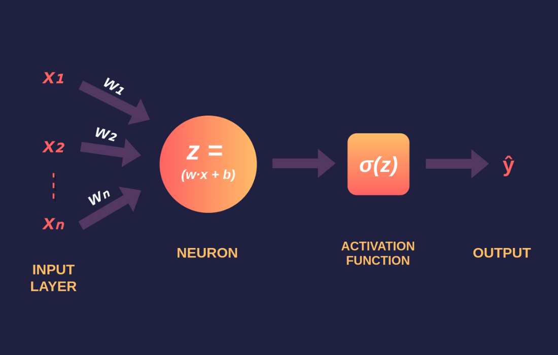
1. Linear Transformation: The first step is applying the weight matrix \( \mathbf{W} \) to the input vector \( \mathbf{x} \), followed by adding a bias \( \mathbf{b} \):
\[
\mathbf{z} = \mathbf{W} \mathbf{x} + \mathbf{b}
\]
where:
– \( \mathbf{z} \) is the intermediate output before applying the activation function.
– \( \mathbf{W} \) is the weight matrix (of dimensions \( m \times n \), where \( m \) is the number of neurons in the next layer and \( n \) is the number of input features).
– \( \mathbf{x} \) is the input vector (of dimension \( n \times 1 \)).
2. Adding Bias: The bias vector \( \mathbf{b} \) ensures that the model can shift the output and thus help with learning the appropriate weights. The bias term has dimensions \( m \times 1 \), and is added to each neuron’s output, shifting the output of the linear transformation.
Thus, the final result of the linear transformation is a vector \( \mathbf{z} \), where each element corresponds to the weighted sum of inputs to a neuron, plus the bias.
—
2.2 Activation Functions
After the linear transformation, we apply an activation function to introduce non-linearity into the model. This step is crucial for allowing the network to learn complex patterns in data. Common activation functions include sigmoid, ReLU, and tanh.
Step-by-Step Derivation of Sigmoid Activation Function
The sigmoid activation function is given by:
\[
\sigma(z) = \frac{1}{1 + e^{-z}}
\]
where \( z \) is the input to the activation function.
1. Derivative of Sigmoid: The derivative of the sigmoid function is required for backpropagation, as it helps compute the gradient of the loss function with respect to the weights. The derivative of \( \sigma(z) \) is:
\[
\frac{d\sigma(z)}{dz} = \sigma(z)(1 – \sigma(z))
\]
This is useful when updating weights during the training process.
Step-by-Step Derivation of ReLU Activation Function
The ReLU (Rectified Linear Unit) activation function is defined as:
\[
\text{ReLU}(z) = \max(0, z)
\]
This means that:
– If \( z > 0 \), then \( \text{ReLU}(z) = z \).
– If \( z \leq 0 \), then \( \text{ReLU}(z) = 0 \).
1. Derivative of ReLU: The derivative of ReLU is:
\[
\frac{d \, \text{ReLU}(z)}{dz} =
\begin{cases}
1 & \text{if } z > 0 \\
0 & \text{if } z \leq 0
\end{cases}
\]
This derivative is very simple and efficient for computing gradients, which is why ReLU is widely used in deep learning.
—
2.3 Loss Functions
The loss function measures how far the neural network’s predictions are from the true values. Minimizing the loss is the primary goal during the training process.
Step-by-Step Derivation of Mean Squared Error (MSE)
For regression tasks, the Mean Squared Error (MSE) is commonly used as a loss function. It is defined as:
\[
L_{\text{MSE}} = \frac{1}{m} \sum_{i=1}^m (y_i – \hat{y}_i)^2
\]
where:
– \( y_i \) is the true value.
– \( \hat{y}_i \) is the predicted value.
– \( m \) is the number of data points.
1. Gradient of MSE Loss: The gradient of the MSE loss function with respect to the predicted output \( \hat{y}_i \) is:
\[
\frac{\partial L_{\text{MSE}}}{\partial \hat{y}_i} = \frac{2}{m} (\hat{y}_i – y_i)
\]
This gradient is used in backpropagation to update the weights during training.
Step-by-Step Derivation of Cross-Entropy Loss
For classification tasks, Cross-Entropy Loss is often used. For binary classification, it is defined as:
\[
L_{\text{CE}} = -\frac{1}{m} \sum_{i=1}^m \left[ y_i \log(\hat{y}_i) + (1 – y_i) \log(1 – \hat{y}_i) \right]
\]
where:
– \( y_i \) is the true label (0 or 1).
– \( \hat{y}_i \) is the predicted probability (output of the sigmoid function).
1. Gradient of Cross-Entropy Loss: The gradient of the cross-entropy loss with respect to the predicted probability \( \hat{y}_i \) is:
\[
\frac{\partial L_{\text{CE}}}{\partial \hat{y}_i} = \frac{\hat{y}_i – y_i}{\hat{y}_i (1 – \hat{y}_i)}
\]
This gradient is used to adjust the weights in the network during backpropagation.
—
2.4 Gradient Descent and Optimization
The goal of training a neural network is to minimize the loss function, and this is achieved using optimization algorithms. The most popular algorithm for training neural networks is gradient descent.
Step-by-Step Derivation of Gradient Descent
Gradient descent updates the weights by moving in the direction of the negative gradient of the loss function with respect to the weights:
\[
\mathbf{W} = \mathbf{W} – \eta \frac{\partial L}{\partial \mathbf{W}}
\]
where:
– \( \mathbf{W} \) is the weight matrix.
– \( \eta \) is the learning rate.
– \( \frac{\partial L}{\partial \mathbf{W}} \) is the gradient of the loss function with respect to the weights.
1. Backpropagation and Weight Update: The gradient \( \frac{\partial L}{\partial \mathbf{W}} \) is computed using backpropagation, which applies the chain rule to compute the gradient for each weight in the network. The gradient for each layer is propagated backwards from the output to the input.
The weight update for layer \( l \) is given by:
\[
\mathbf{W}^{(l)} = \mathbf{W}^{(l)} – \eta \frac{\partial L}{\partial \mathbf{W}^{(l)}}
\]
where \( \mathbf{W}^{(l)} \) represents the weights at layer \( l \).
—
3. Backpropagation: Step-by-Step Derivation
Backpropagation is an essential algorithm for training neural networks, as it computes the gradient of the loss function with respect to each weight. Here’s how backpropagation works mathematically:
1. Forward Pass: Compute the output of each layer in the network using the weight matrix, bias, and activation function. For a given layer \( l \):
\[
\mathbf{z}^{(l)} = \mathbf{W}^{(l)} \mathbf{a}^{(l-1)} + \mathbf{b}^{(l)}
\]
\[\mathbf{a}^{(l)} = \sigma(\mathbf{z}^{(l)})
\]
2. Compute the Loss Gradient: Compute the derivative of the loss with respect to the output of the network (for the last layer). If the loss function is cross-entropy, for the last layer:
\[
\frac{\partial L}{\partial \mathbf{a}^{(L)}} = \hat{\mathbf{y}} – \mathbf{y}
\]
3. Backward Pass: For each layer, starting from the output layer, propagate the gradient backwards using the chain rule. For each hidden layer \( l \), the gradient with respect to the weights is:
\[
\frac{\partial L}{\partial \mathbf{W}^{(l)}} = \frac{\partial L}{\partial \mathbf{a}^{(l)}} \cdot \frac{\partial \mathbf{a}^{(l)}}{\partial \mathbf{z}^{(l)}} \cdot \frac{\partial \mathbf{z}^{(l)}}{\partial \mathbf{W}^{(l)}}
\]
This process continues backward through the network until all gradients are computed.
4. Update Weights: Finally, update the weights using gradient descent:
\[
\mathbf{W}^{(l)} = \mathbf{W}^{(l)} – \eta \frac{\partial L}{\partial \mathbf{W}^{(l)}}
\]
—
4. Conclusion
Neural networks are powerful tools for machine learning, and their success is deeply rooted in the mathematical concepts of linear algebra, calculus, and optimization. From matrix multiplications to activation functions and gradient descent, each mathematical component plays a vital role in allowing neural networks to learn from data and make accurate predictions.
This blog has provided a detailed, step-by-step derivation of key formulas used in neural networks, from linear transformations to backpropagation. Understanding the mathematics behind neural networks is essential for building and optimizing these models for real-world applications.


