Algorithm design and analysis form the backbone of computer science and computational theory. Algorithms are step-by-step procedures or formulas for solving problems, and their efficiency determines how well software performs in terms of speed, memory usage, and scalability. Mathematics plays a pivotal role in both designing algorithms and analyzing their performance. This blog explores the mathematical principles involved in designing and analyzing algorithms, diving into topics such as time and space complexity, recurrence relations, algorithm design paradigms, and more.
1. Introduction to Algorithm Design
In algorithm design, the goal is to create a step-by-step procedure that solves a computational problem in the most efficient manner possible. Efficiency is typically measured in terms of time complexity (how quickly an algorithm runs) and space complexity (how much memory the algorithm consumes). These measures are crucial when dealing with large datasets or when real-time performance is required.
Mathematics provides the necessary tools for both designing algorithms and analyzing their efficiency. The mathematical techniques used in algorithm design include:
– Asymptotic Notation (Big-O, Big-Theta, and Big-Omega)
– Recurrence Relations
– Probability and Combinatorics
– Linear Algebra and Matrix Theory
– Graph Theory
– Optimization Techniques
In this blog, we will explore these techniques in detail with examples and provide the necessary mathematical derivations to support each one.
—
2. Asymptotic Analysis: Time and Space Complexity
Asymptotic analysis is used to evaluate the growth rate of an algorithm’s time and space complexity as the input size increases. This helps us understand the efficiency of an algorithm in the long run, independent of machine-dependent constants.
2.1 Time Complexity and Big-O Notation
Time complexity refers to how the execution time of an algorithm scales with the input size \( n \). The most common notation for analyzing time complexity is Big-O notation.
Big-O Notation:
Big-O describes an upper bound on the time complexity of an algorithm, ensuring that the algorithm will never take longer than a specified function of the input size. For an algorithm with time complexity \( T(n) \), we write:
\[
T(n) = O(f(n)) \quad \text{if there exists constants } c > 0 \text{ and } n_0 \text{ such that for all } n > n_0, \, T(n) \leq c \cdot f(n)
\]
Examples of Common Time Complexities:
– Constant time: \( O(1) \) — The execution time does not depend on the input size. Example: Accessing an element in an array by index.
– Linear time: \( O(n) \) — The execution time grows linearly with the input size. Example: Searching for an element in an unsorted list.
– Quadratic time: \( O(n^2) \) — The execution time grows quadratically. Example: Bubble sort or selection sort.
– Logarithmic time: \( O(\log n) \) — The execution time grows logarithmically with input size. Example: Binary search.
Example: Linear Search
Consider a linear search algorithm that searches for an element \( x \) in an unsorted list of size \( n \). In the worst case, the algorithm has to check every element, so its time complexity is \( O(n) \).
2.2 Space Complexity
Space complexity refers to how much memory an algorithm requires as a function of the input size \( n \). Like time complexity, space complexity is often analyzed using Big-O notation.
Example: Space Complexity of an Algorithm
Consider an algorithm that takes an array of size \( n \) and creates a new array to store its result. The space complexity of this algorithm would be \( O(n) \), since it requires space proportional to the size of the input.
—
3. Recurrence Relations in Algorithm Design
A recurrence relation is an equation that recursively defines a sequence of values in terms of previous terms. In algorithm analysis, recurrence relations are used to express the running time of recursive algorithms.
3.1 Solving Recurrence Relations
Consider an algorithm that divides a problem of size \( n \) into \( k \) subproblems, each of size \( n/a \), and takes \( O(n^d) \) time to divide the problem and combine the solutions. The recurrence relation for this algorithm is:
\[
T(n) = k \cdot T\left(\frac{n}{a}\right) + O(n^d)
\]
We solve this recurrence using several methods, including the **Master Theorem**, **Recursion Tree Method, and Substitution Method.
3.2 Example: Merge Sort
Merge Sort is a classic example of a divide-and-conquer algorithm. The recurrence relation for Merge Sort is:
\[
T(n) = 2T\left(\frac{n}{2}\right) + O(n)
\]
Using the Master Theorem, we compare the recurrence to the general form:
\[
T(n) = aT\left(\frac{n}{b}\right) + O(n^d)
\]
In the case of Merge Sort, \( a = 2 \), \( b = 2 \), and \( d = 1 \). According to the Master Theorem, we calculate \( \log_b a = \log_2 2 = 1 \).
Since \( d = \log_b a \), the time complexity is \( O(n \log n) \).
Thus, the time complexity of Merge Sort is \( O(n \log n) \).
—
4. Algorithm Design Paradigms
In algorithm design, we often use certain paradigms or techniques that guide the development of algorithms. These include:
– Divide and Conquer
– Greedy Algorithms
– Dynamic Programming
– Backtracking
– Branch and Bound
4.1 Divide and Conquer
In the Divide and Conquer paradigm, we break the problem into smaller subproblems, solve the subproblems recursively, and then combine the solutions.
Example: Merge Sort (Already discussed)
The recurrence relation for Merge Sort, \( T(n) = 2T\left(\frac{n}{2}\right) + O(n) \), is solved using divide-and-conquer.
4.2 Greedy Algorithms
Greedy algorithms make local optimal choices at each step, with the hope of finding a global optimum.
Example: Activity Selection Problem
Given a set of activities, each with a start and finish time, the goal is to select the maximum number of non-overlapping activities. A greedy approach selects the activity that finishes the earliest at each step.
The algorithm works as follows:
1. Sort the activities by finish time.
2. Select the first activity and then repeatedly select the next activity whose start time is greater than or equal to the finish time of the previously selected activity.
The time complexity of this algorithm is dominated by the sorting step, so it is \( O(n \log n) \).
4.3 Dynamic Programming
Dynamic programming (DP) is used for problems that can be broken down into overlapping subproblems. In DP, we solve each subproblem once and store its solution to avoid redundant calculations.
Example: Fibonacci Sequence
The recursive definition of the Fibonacci sequence is:
\[
F(n) = F(n-1) + F(n-2)
\]
A naive recursive solution has exponential time complexity, \( O(2^n) \). However, using dynamic programming (memoization), we can compute the Fibonacci sequence in linear time:
\[
F(n) = O(n)
\]
—
5. Graph Theory in Algorithms
Graphs are mathematical structures used to model relationships between objects. In algorithm design, graphs are used in a wide variety of applications, including network flow, shortest path algorithms, and scheduling problems.
5.1 Shortest Path Algorithms
One of the most famous algorithms for finding the shortest path in a graph is Dijkstra’s Algorithm. The algorithm finds the shortest path from a source node to all other nodes in a weighted graph.
The key steps of Dijkstra’s Algorithm are:
1. Initialize the distance to the source node as 0 and all other nodes as infinity.
2. Iteratively select the node with the smallest known distance and update its neighbors.
The time complexity of Dijkstra’s Algorithm using a priority queue is \( O(E \log V) \), where \( E \) is the number of edges and \( V \) is the number of vertices.
5.2 Minimum Spanning Tree
The Minimum Spanning Tree (MST) of a graph is a subset of edges that connects all vertices without any cycles and with the minimum possible total edge weight. Kruskal’s Algorithm and Prim’s Algorithm are two famous algorithms for finding the MST.
– Prim’s Algorithm: Works by growing the MST one vertex at a time, starting with an arbitrary vertex.
– Kruskal’s Algorithm: Works by sorting all the edges and adding them to the MST in increasing order of weight, ensuring no cycles are formed.
Both algorithms have a time complexity of \( O(E \log V) \) using appropriate data structures.
—
6. Optimization and Linear Programming
Optimization is about finding the best solution from a set of feasible solutions, and it plays a central role in many algorithms.
6.1 Linear Programming
Linear programming is a mathematical technique used to find the best outcome in a mathematical model with linear constraints. The standard form of a linear programming problem is:
\[
\text{Maximize } \mathbf{c}^T \mathbf{x}
\]
\[
\text{Subject to: } A \mathbf{x} \leq \mathbf{b}, \, \mathbf{x} \geq 0
\]
Here, \( \mathbf{x} \) is a vector of decision variables, \( A \) is a matrix of coefficients, and \( \mathbf{c} \) is the vector of coefficients for the objective function. The solution to the linear programming problem can be found using Simplex Algorithm or Interior Point Methods.
—
7. Conclusion
Mathematics is not just the language of algorithms but also the framework that makes algorithm design and analysis effective. From the use of asymptotic analysis to recurrence relations, optimization, and graph theory, mathematical techniques are indispensable tools in the field of algorithm design. Understanding these mathematical foundations allows algorithm designers to create efficient and scalable solutions to a wide range of computational problems.
By combining theoretical principles with practical techniques, one can build powerful algorithms that tackle everything from simple problems to complex, real-world applications. This mathematical rigor enables the development of algorithms that can handle vast amounts of data efficiently and effectively.


