


 and How Data Passes Through Them")


, and Neural Networks in a structured way")
")

 That You’ll Want to Buy for yourself")


Course Introduction: How Large Language Models (LLMs) Work
What You Will Learn: The LLM Processing Pipeline
In this course, you will learn how Large Language Models (LLMs) process text step by step, transforming raw input into intelligent predictions. Here’s a visual overview of the journey your words take through an LLM:
Module Roadmap
You will explore each step in detail:
1. Input Text: How the raw text enters the model.
2. Tokenization: How text is split into tokens the model can process.
3. Embedding: How each token is turned into a numerical vector.
4. Self-Attention (Q, K, V): How the model represents each token’s role and context.
5. QKV Computation: How attention weights are calculated and applied.
6. Activation Functions: How the model introduces non-linearity and learns complex patterns.
7. Weighted Sum: How the model builds new representations using attention.
8. New Token Vector: The updated understanding of each token.
9. Predicted Word: How the model produces its output.
By the end of this course, you’ll understand every stage in the LLM pipeline and how they work together to turn your text into smart, context-aware predictions.
|
1 2 3 4 5 6 7 8 9 10 11 12 13 14 15 16 17 18 19 20 21 22 23 24 25 26 27 28 29 30 31 32 33 34 35 36 37 38 39 40 41 42 43 44 45 46 47 48 49 50 51 52 53 54 55 56 57 58 59 60 61 62 63 64 65 66 67 68 |
+-------------------+ | Input Text | +-------------------+ | | v +---------------------+ | Tokenization | | (Split into | | individual words) | +----------------- --+ | | v +--------------------+ | Embedding | | (Convert words | | into numerical | | representations) | +--------------------+ | | v +--------------------+ | Self-Attention | | (Compute Q, K, V) | +--------------------+ | | v +----------------------+ | QKV Computation | | (Compute attention | | weights and apply) | +----------------------+ | | v +-------------------+ | Activation | | Function (e.g., | | ReLU, GELU) | +-------------------+ | | v +---------------------+ | Weighted Sum | | (Compute weighted | | sum of attention) | +---------------------+ | | v +------------------------+ | New Token Vector | | (Output of self- | | attention mechanism) | +------------------------+ | | v +--------------------+ | Predicted Word | | (Output of model) | +--------------------+ |
Input Text:
What are Examples of Large Language Model Data?
Examples of LLM data include:
- Books and Literature: Digitized versions of works across various genres.
- News Articles: Articles from newspapers, magazines, and online news platforms covering a wide range of topics.
- Websites: Text from blogs, forums, and social media platforms that provide diverse conversational.
- Scientific Papers: Research papers and journals that offer specialized and technical language data.
What Data Type is Large Language Model Data?
Large Language Model (LLM) data includes various data types essential for AI training:
- Textual Data: This forms the backbone of LLMs. It includes written content like books, articles, websites, and social media posts, as well as numerical data such as vectors, matrices, and tensors.
- Structured Data: Sometimes, models utilize data from structured formats like databases, tables, or CSV files, especially for tasks involving structured text.
- Metadata: Additional information about the text, such as the source, publication date, and author.
- Tokenized Data: Text is broken down into tokens—words, subwords, or characters. These tokens are the basic units for the LLM learning process.
- Training Labels: In supervised learning, labeled data pairs each text piece with a label or category. This helps in tasks like classification, named entity recognition, and sentiment analysis.
To train Large Language Models (LLMs) for diverse tasks like math, story writing, coding, and more, the input data comes in a variety of formats and structures, depending on the task type, data source, and training pipeline. Here’s a structured overview:
TYPES OF DATA USED TO TRAIN LLMs:
1. Text Data (Plaintext / Tokenized)
Used for:
- General language modeling
- Story writing
- Dialogues and conversations
Format examples:
.txtfiles from books, web pages, Wikipedia, Common Crawl, etc.- JSONL (
.jsonl) lines where each line is a separate document or conversation.
|
1 2 3 4 |
{"text": "Once upon a time in a far away kingdom..."} {"text": "In this lesson, we will cover Newton's laws of motion."} |
2. Math Data
Used for:
- Solving symbolic math, word problems, equation understanding
Sources & Format:
- LaTeX math problems (
.tex) - Structured datasets:
Example (JSON):
|
1 2 3 4 5 6 |
{ "question": "What is 15% of 80?", "answer": "0.15 * 80 = 12" } |
3. Programming / Code Data
Used for:
- Code generation, debugging, explaining code
Formats:
.py,.js,.cpp, etc.- JSONL with input-output pairs from GitHub, StackOverflow, etc.
Example:
|
1 2 3 4 5 6 |
{ "prompt": "Write a Python function to compute factorial.", "completion": "def factorial(n):\n if n==0: return 1\n return n * factorial(n-1)" } |
4. Dialog / Instruction Data
Used for:
-
Chat models, instruction tuning (e.g., ChatGPT, Claude)
Format: JSON / JSONL / Markdown
|
1 2 3 4 5 6 |
{ "instruction": "Explain gravity like I'm 5", "response": "Gravity is like a magnet that pulls everything down to the ground..." } |
5. Structured Tables and CSVs
Used for:
-
Training on data tables, data analysis, QA on tables
Format:
.csv,.tsvor tabular JSON
|
1 2 3 4 5 |
Name, Age, Grade Alice, 12, A Bob, 13, B |
or
|
1 2 3 4 5 6 7 8 9 10 |
{ "table": { "columns": ["Name", "Age", "Grade"], "data": [["Alice", 12, "A"], ["Bob", 13, "B"]] }, "question": "Who got grade A?", "answer": "Alice" } |
6. Multimodal Inputs (Images, Videos, Diagrams)
Used for:
-
Visual question answering, code-in-the-wild, scientific figures
Format:
- Base64 images + captions in JSON
- Videos split into frames + text transcriptions
- JSONL combining modalities
Table Overview
| Task Type | Common Input Formats | Examples |
|---|---|---|
| Story Writing | .txt, .jsonl | Books, fanfiction, news |
| Math Problems | .json, LaTeX, .txt | GSM8K, MATH |
| Code Completion | .py, .jsonl | GitHub, StackOverflow dumps |
| Conversations | .jsonl, .md, dialogue trees | Chat logs, instruction-response |
| Tabular Reasoning | .csv, structured JSON | Excel exports, data tables |
| Multimodal Tasks | JSON + Base64 / image paths | VQA, math with diagrams |
LLM Training Data: The 8 Main Public Data Sources
The biggest challenge in training large language models (LLMs) isn’t their architecture-it’s finding high-quality, diverse, and unbiased data in a vast and noisy digital landscape. This is true whether you’re building an LLM from scratch or fine-tuning a pre-trained one, as you’ll need to use high-quality data compiled from multiple sources.
Main public data sources for LLMs
Building a custom training dataset will require an effective web scraping tool that can handle various page types and stringent anti-scraping systems. One way is to develop a custom web scraping infrastructure, or alternatively, you can choose a web scraping API that’s specifically designed to extract data from difficult websites. Before going with one or the other option, you should compile a list of public data sources you want to scrape. See the list below to get a general overview:
1. Web pages
This entails any domain-specific content, including websites focused on science, retail, business, etc. Depending on your use case, websites for LLM training include:
-
Specific public content on any website, like blog posts, articles, and reviews.
-
Search engine results from Google, Bing, and other engines.
-
E-commerce data from Amazon, Google Shopping, and similar large retail sites.
2. Books
Public domain sources like Project Gutenberg and similar provide a wealth of quality data, covering a diverse range of topics and writing styles found in books.
3. Community networks
Public access community networks, forums, and social media platforms are perfect for conversational and humanistic texts. Platforms like Stack Exchange also offer deep knowledge of various topics like mathematics, physics, linguistics, programming, and others.
4. Science and research sources
If you want to train your LLM on scientific data, consider sources like Google Scholar, PLOS ONE, DOAJ, PubMed Central® (PMC), and similar platforms that provide multiple documents that are peer-reviewed.
5. News outlets
To train an LLM proficient in current international and national events, politics, and other fields, you may want to feed it with public news data gathered from Google News and similar platforms.
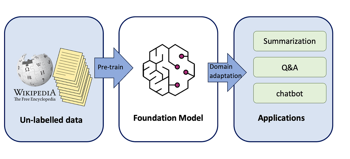
6. Wikipedia
This free online encyclopedia hosts around 6.8 million content pages with around 4.7 billion words, covering almost any topic. While it’s not the most reliable source since anyone can edit the content, it’s still a great source for LLM training due to its well-written and multilingual text with wide topic coverage. For a well-rounded LLM, Wikipedia should be supplemented with more data from other datasets, similar to how OpenAI’s GPT-3 and Google’s BERT were trained.
7. Code sources
If your goal is to train an LLM that can navigate different programming nuances and generate code that works using different programming languages, then consider using public sources like GitHub, Stackhare, DockerHub, and Kaggle.
8. Video platforms
Public video platforms are a great source of conversational text for LLM training. In essence, you would need to use available transcribed video texts.
Common Crawl maintains a free, open repository of web crawl data that can be used by anyone.
Tokenization
What Is Tokenization?
Tokenization, in a general sense, is the process of replacing sensitive data with a non-sensitive equivalent called a token. This process is used in various fields, including data security, natural language processing (NLP), and financial transactions, to protect information, improve data processing, and enhance the security of systems.
We have come so far from the traditional NLTK tokenization process. And though we have state-of-the-art algorithms for tokenization, it’s always a good practice to understand its evolution and how we got to where we are now.
So, here’s what we’ll cover:
- Why do we need a tokenizer?
- Types of tokenization – Word, Character, and Subword.
- Byte Pair Encoding Algorithm – a version of which is used by most NLP models these days.
In deep learning, tokenization is the process of converting a sequence of characters into a sequence of tokens which further needs to be converted into a sequence of numerical vectors that can be processed by a neural network. Tokenization in Large Language Models (LLMs): A Complete Guide
Example Sentence
Input: "Cats sleep on mats."
“Cats sleep on mats.” is tokenized by different tokenization methods used in modern LLMs:
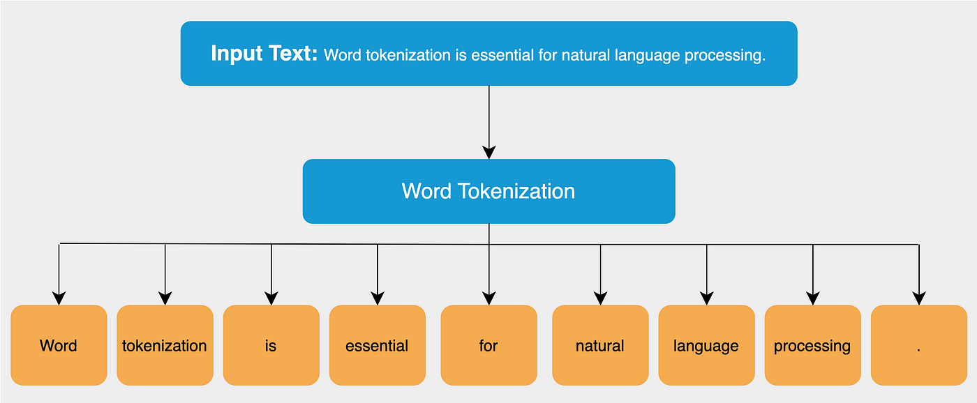
1. Word-Level Tokenizer
Splits by whitespace and punctuation.
|
1 2 3 |
["Cats", "sleep", "on", "mats", "."] |
2. Byte-Pair Encoding (BPE)
(Used in GPT-2, GPT-3, GPT-4, LLaMA, etc.)
|
1 2 3 |
["Cats", " sleep", " on", " mats", "."] |
Note: Leading space included for all tokens after the first (used to preserve whitespace context).
3. WordPiece Tokenizer
(Used in BERT, DistilBERT, RoBERTa, etc.)
|
1 2 3 |
["cats", "sleep", "on", "mat", "##s", "."] |
"mats"is split into root"mat"and suffix"##s".
4. SentencePiece (Unigram/BPE)
(Used in T5, XLNet, ALBERT, LLaMA-2)
|
1 2 3 |
["▁Cats", "▁sleep", "▁on", "▁mats", "."] |
The
▁prefix represents a space before the word. SentencePiece learns tokens including space context.
GPT-2 Tokenization (Byte-Pair Encoding)
GPT-2 uses Byte-Pair Encoding (BPE). It learns the most frequent pairs of characters in the dataset and merges them. Also, leading spaces matter in GPT-style tokenizers.
| Token | Meaning | Token ID |
|---|---|---|
| 'Cats' | The word "Cats" with no leading space | 17871 |
| ' sleep' | Space + "sleep" | 1024 |
| ' on' | Space + "on" | 319 |
| ' mats' | Space + "mats" | 11491 |
| '.' | Period | 13 |
Visualization:
|
1 2 3 4 5 |
| 'Cats' | ' sleep' | ' on' | ' mats' | '.' | |--------|----------|-------|---------|-----| | 17871 | 1024 | 319 | 11491 | 13 | |
GPT-2 keeps most words intact but adds leading spaces to non-initial tokens.
BERT Tokenization (WordPiece)
BERT uses WordPiece, which splits unknown or rare words into subword units and always lowercases the input (uncased model).
| Token | Meaning | Token ID |
|---|---|---|
| [CLS] | Start of sentence | 101 |
| 'cats' | Lowercased version of "Cats" | 4937 |
| 'sleep' | Recognized word | 8811 |
| 'on' | Recognized word | 2006 |
| 'mat' | Root word split from "mats" | 8818 |
| '##s' | BERT-style suffix for subword "s" | 2015 |
| '.' | Period | 1012 |
| [SEP] | End of sentence | 102 |
|
1 2 3 4 5 |
| [CLS] | 'cats' | 'sleep' | 'on' | 'mat' | '##s' | '.' | [SEP] | |-------|--------|---------|------|-------|-------|-----|--------| | 101 | 4937 | 8811 | 2006 | 8818 | 2015 | 1012| 102 | |
BERT splits words like “mats” into mat + ##s, preserving morphology while reducing vocabulary size.
| Feature | GPT-2 | BERT |
|---|---|---|
| Tokenizer Type | Byte-Pair Encoding (BPE) | WordPiece |
| Handles unknown words | With frequent subword units | With ##subwords |
| Space-sensitive? | Yes (leading space = token) | No |
| Special tokens | No special tokens by default | [CLS], [SEP] added |
| Output Token IDs | Raw integer IDs | Raw integer IDs with specials |
Embedding
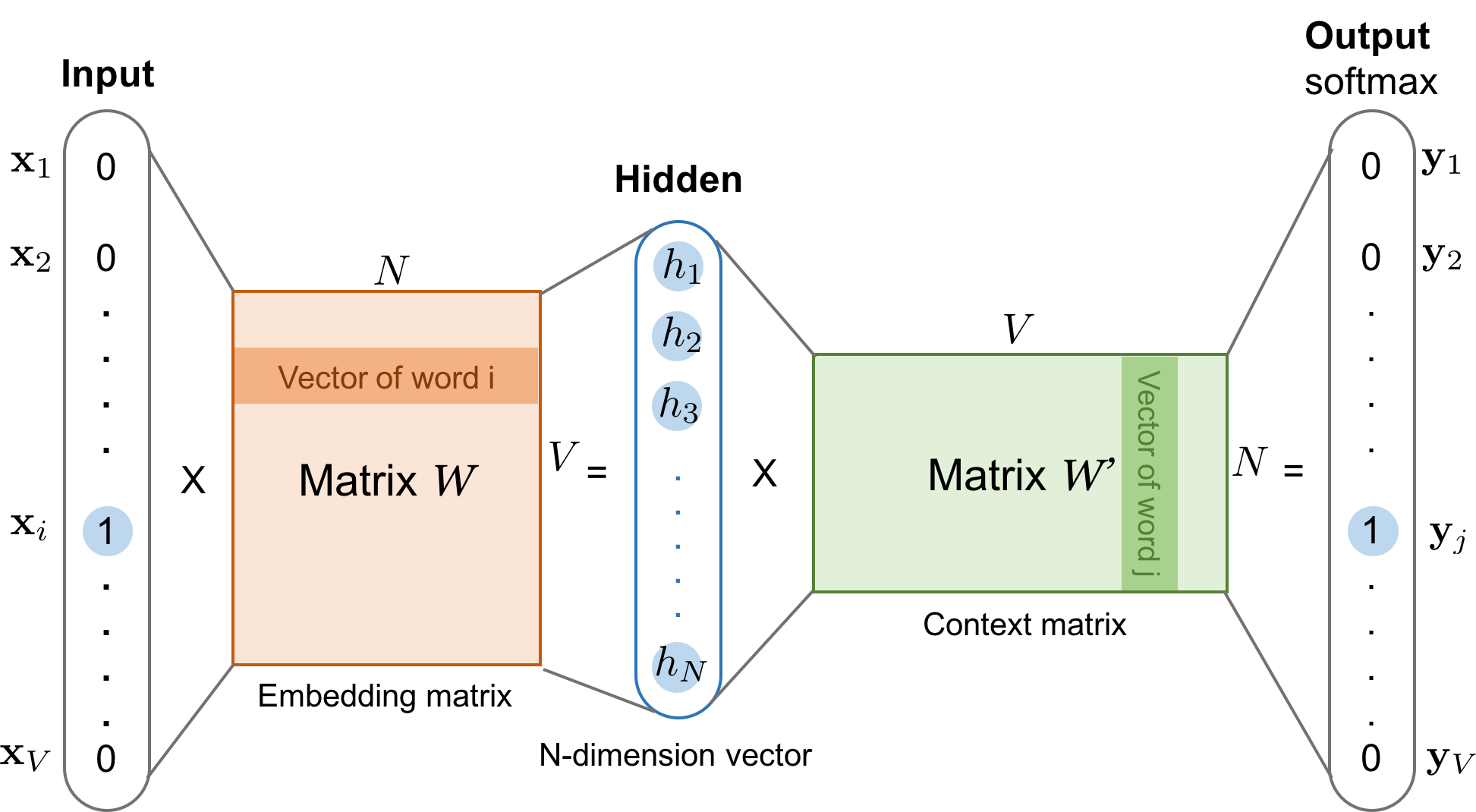
What is the Embedding Matrix?
The embedding matrix is a large table of numbers with:
– Rows: One for each token in the vocabulary (e.g., 50,000 tokens).
– Columns: The embedding size (e.g., 768 features per token).
Each row in this matrix represents the vector for a specific token ID.
|
1 2 3 4 5 6 7 8 9 10 11 |
"cats sleep." ↓ ['[CLS]', 'cats', 'sleep', '.', '[SEP]'] ↓ [101, 4937, 8811, 1012, 102] ↓ → Lookup in [30522 x 768] embedding matrix ↓ → [5 x 768] token embeddings |
Visual Representation
Suppose:
– Vocabulary size: 5 tokens (for simplicity)
– Embedding size: 4 (real models use hundreds)
Embedding Matrix Example:
The embedding matrix is a big table (matrix) where:
– Each row corresponds to a token ID.
– Each row contains a vector of numbers (the “embedding”) that represents that token’s meaning for the model.
|
1 2 3 4 5 6 7 8 9 |
| Token | Token ID | Embedding Vector (Row) | |-------|----------|----------------------------------| | the | 0 | `[ 0.12, -0.15, 0.03, 0.77 ]` | | cat | 1 | `[ 0.45, 0.22, -0.56, 0.18 ]` | | sat | 2 | `[ 0.31, -0.08, 0.14, 0.65 ]` | | on | 3 | `[ -0.27, 0.12, 0.41, -0.09 ]` | | mat | 4 | `[ 0.02, 0.67, -0.31, 0.33 ]` | |

How Does the Mapping Work?
Think of the embedding matrix like a spreadsheet:
– Row 0: Embedding for token ID 0
– Row 1: Embedding for token ID 1
Summary:
– Each token ID directly points to a row in the embedding matrix.
– The mapping is a simple lookup: token ID n maps to the nth row of the embedding matrix.
– This gives the model a numerical vector for each token, which it uses for further processing.
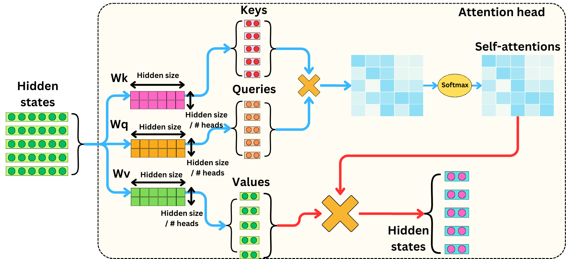
Self–Attention (Compute Q, K, V)
In the self-attention mechanism, Query (Q), Key (K), and Value (V) are matrices used to compute attention weights and contextualized representations of tokens in a sequence. Q represents what a token is seeking, K represents what’s relevant to Q, and V contains the actual information to be retrieved.
Input Vectors and Weight Matrices: Mathematical Visualization
Each token is first mapped to an embedding vector (from the embedding matrix).
For a single token with embedding vector \( X \), the model computes three new vectors—Query (Q), Key (K), Value (V)—using matrix multiplication with learned parameters.
\[
\begin{gather}
\textbf{Q} = \textbf{X} \cdot \mathbf{W}^Q \\
\textbf{K} = \textbf{X} \cdot \mathbf{W}^K \\
\textbf{V} = \textbf{X} \cdot \mathbf{W}^V
\end{gather}
\]
Where:
– \( \textbf{X} \) is the input embedding vector of shape \( 1 \times d_{\text{model}} \)
– \( \mathbf{W}^Q, \mathbf{W}^K, \mathbf{W}^V \) are weight matrices of shape \( d_{\text{model}} \times d_k \) (or \( d_v \) for V)
– \( d_{\text{model}} \) is the embedding dimension (e.g., 768)
– \( d_k \) is the size of query/key vectors (e.g., 64)
– \( d_v \) is the size of value vectors (often same as \( d_k \))
For a batch of tokens (sequence):
Suppose you have \( N \) tokens, stacked as a matrix \( \mathbf{X} \) of shape \( N \times d_{\text{model}} \):
\[
\begin{gather}
\mathbf{Q} = \mathbf{X} \cdot \mathbf{W}^Q \\
\mathbf{K} = \mathbf{X} \cdot \mathbf{W}^K \\
\mathbf{V} = \mathbf{X} \cdot \mathbf{W}^V
\end{gather}
\]
Where:
– \( \mathbf{Q}, \mathbf{K}, \mathbf{V} \) are matrices of shape \( N \times d_k \) (or \( N \times d_v \) for V)
– Each row corresponds to a token in the sequence.
Visual Example:
If
– \( \mathbf{X} = \begin{bmatrix} x_1 \\ x_2 \\ x_3 \end{bmatrix} \) (token embeddings, \( 3 \times d_{\text{model}} \))
– \( \mathbf{W}^Q, \mathbf{W}^K, \mathbf{W}^V \) (\( d_{\text{model}} \times d_k \))
Then
\[
\begin{gather}
\mathbf{Q} =
\begin{bmatrix} x_1 \\ x_2 \\ x_3 \end{bmatrix}
\cdot
\mathbf{W}^Q
=
\begin{bmatrix} q_1 \\ q_2 \\ q_3 \end{bmatrix}
\end{gather}
\]
where each \( q_i \) is the query vector for token \( i \).
Let’s walk through a complete mathematical example of self-attention using provided token embeddings. We’ll assume:
– Embedding dimension \( d = 4 \)
– Single attention head for simplicity
– Learned weight matrices \( W^Q, W^K, W^V \in \mathbb{R}^{4 \times 3} \) (we’ll use \( d_k = d_v = 3 \) for illustration)
NOTE: a 4-column × 3-column matrix multiplication is possible only if the number of rows in the second matrix equals the number of columns in the first.
1. Input Embeddings (X)
\[
X = \begin{bmatrix}
\text{the} & 0.12 & -0.15 & 0.03 & 0.77 \\
\text{cat} & 0.45 & 0.22 & -0.56 & 0.18 \\
\text{sat} & 0.31 & -0.08 & 0.14 & 0.65 \\
\text{on} & -0.27 & 0.12 & 0.41 & -0.09 \\
\text{mat} & 0.02 & 0.67 & -0.31 & 0.33 \\
\end{bmatrix}
\]
2. Learned Weight Matrices (Random Initialization)
\[
W^Q = \begin{bmatrix}
0.1 & -0.2 & 0.3 \\
0.4 & 0.0 & -0.1 \\
-0.2 & 0.3 & 0.1 \\
0.0 & 0.1 & 0.2 \\
\end{bmatrix}\]
\[
W^K = \begin{bmatrix}
0.2 & 0.1 & -0.1 \\
0.3 & 0.0 & 0.2 \\
-0.1 & 0.2 & 0.0 \\
0.1 & -0.1 & 0.3 \\
\end{bmatrix}\]
\[
W^V = \begin{bmatrix}
0.0 & 0.1 & -0.2 \\
0.2 & -0.1 & 0.3 \\
0.1 & 0.0 & 0.2 \\
-0.1 & 0.2 & 0.1 \\
\end{bmatrix}
\]
3. Compute Q, K, V Matrices
Query (Q):
\[
Q = X W^Q = \begin{bmatrix}
0.12\times0.1 + (-0.15)\times0.4 + \cdots & \cdots & \cdots \\
\vdots & \ddots & \vdots \\
\end{bmatrix}
\]
\[
Q = \begin{bmatrix}
-0.021 & 0.069 & 0.231 \\
0.127 & -0.192 & -0.119 \\
0.052 & 0.027 & 0.236 \\
-0.131 & 0.165 & 0.037 \\
0.269 & -0.067 & -0.049 \\
\end{bmatrix}
\]
Key (K):
\[
K = X W^K = \begin{bmatrix}
0.12\times0.2 + (-0.15)\times0.3 + \cdots & \cdots & \cdots \\
\vdots & \ddots & \vdots \\
\end{bmatrix}
\]
\[
K = \begin{bmatrix}
-0.021 & 0.119 & 0.221 \\
0.052 & -0.061 & 0.043 \\
0.089 & 0.038 & 0.181 \\
0.008 & 0.149 & -0.129 \\
0.255 & -0.073 & 0.063 \\
\end{bmatrix}
\]
Value (V):
\[
V = X W^V = \begin{bmatrix}
0.12\times0.0 + (-0.15)\times0.2 + \cdots & \cdots & \cdots \\
\vdots & \ddots & \vdots \\
\end{bmatrix}
\]
\[
V = \begin{bmatrix}
-0.041 & 0.167 & 0.037 \\
-0.119 & 0.092 & 0.148 \\
-0.012 & 0.187 & 0.201 \\
0.104 & 0.022 & 0.129 \\
0.053 & 0.223 & -0.031 \\
\end{bmatrix}
\]
4. Compute Attention Scores
\[
\text{Scores} = \frac{QK^\top}{\sqrt{d_k}} = \frac{1}{\sqrt{3}} \begin{bmatrix}
q_{\text{the}} \cdot k_{\text{the}} & q_{\text{the}} \cdot k_{\text{cat}} & \cdots \\
\vdots & \ddots & \vdots \\
\end{bmatrix}
\]
Example Calculation for \( q_{\text{cat}} \cdot k_{\text{sat}} \):
\[
0.127 \times 0.089 + (-0.192) \times 0.038 + (-0.119) \times 0.181 = -0.037
\]
Full Scores Matrix:
\[
\frac{1}{\sqrt{3}} \begin{bmatrix}
0.071 & -0.037 & 0.066 & -0.016 & 0.006 \\
-0.037 & 0.035 & -0.016 & -0.052 & -0.069 \\
0.066 & -0.016 & 0.058 & 0.010 & -0.023 \\
-0.016 & -0.052 & 0.010 & 0.056 & 0.026 \\
0.006 & -0.069 & -0.023 & 0.026 & 0.089 \\
\end{bmatrix}
\]
5. Apply Softmax

Row-wise softmax converts scores to probabilities:
\[
\text{Attention Weights} = \text{softmax}(\text{Scores}) = \begin{bmatrix}
0.23 & 0.19 & 0.22 & 0.18 & 0.18 \\
0.17 & 0.22 & 0.18 & 0.16 & 0.27 \\
0.23 & 0.18 & 0.22 & 0.19 & 0.18 \\
0.18 & 0.16 & 0.19 & 0.23 & 0.24 \\
0.19 & 0.16 & 0.18 & 0.22 & 0.25 \\
\end{bmatrix}
\]
6. Compute Weighted Values
\[
\text{Output} = \text{Attention Weights} \cdot V = \begin{bmatrix}
\sum_j \alpha_{1j} v_j \\
\vdots \\
\sum_j \alpha_{5j} v_j \\
\end{bmatrix}
\]
First Row (“the” token output):
\[
0.23 \times \begin{bmatrix}-0.041\\0.167\\0.037\end{bmatrix} + 0.19 \times \begin{bmatrix}-0.119\\0.092\\0.148\end{bmatrix} + \cdots = \begin{bmatrix}-0.027\\0.142\\0.112\end{bmatrix}
\]
Final Output:
\[
\begin{bmatrix}
-0.027 & 0.142 & 0.112 \\
-0.038 & 0.156 & 0.131 \\
-0.025 & 0.150 & 0.123 \\
-0.016 & 0.138 & 0.138 \\
-0.012 & 0.145 & 0.129 \\
\end{bmatrix}
\]
Key Observations:
1. Dynamic Attention: “cat” pays most attention to “mat” (weight = 0.27).
2. Information Mixing: Each output token combines information from all tokens.
3. Dimensionality: Output preserves the original sequence length (\( 5 \times 3 \)).
This demonstrates how self-attention dynamically reweights token representations based on their relationships. For multi-head attention, this process runs in parallel with different \( W^Q, W^K, W^V \) per head.
Multi-Head Attention Extension
So far, we’ve computed self-attention using a single head, which gives the model one way to focus on relationships between tokens. But what if one head isn’t enough?
Why Multi-Head Attention?
Each attention head captures a different aspect of relationships between words. For example:
-
One head might focus on syntactic structure,
-
Another on semantic similarity,
-
Yet another on positional dependencies.
Single-head attention gives the model one view of the input. But real understanding often needs multiple perspectives. This is where multi-head attention comes in.
Step 1: Parallel QKV Computation per Head
We compute separate $Q,K,V$ matrices per head using different learned weight matrices:
\[
Q_i = X W_i^Q, \quad K_i = X W_i^K, \quad V_i = X W_i^V
\]
For each head $i$, the attention is computed independently:
\[
\text{head}_i = \text{Attention}(Q_i, K_i, V_i) = \text{softmax}\left( \frac{Q_i K_i^\top}{\sqrt{d_k}} \right) V_i
\]
Each head gives an output matrix of shape $n \times d_v$.
Step 2: Concatenate the Outputs
Once all heads produce their respective outputs, we concatenate them along the feature dimension:
\[
\text{MultiHeadOutput} = \text{Concat}(\text{head}_1, \ldots, \text{head}_h)
\]
For example, with 2 heads each producing outputs of shape $5 \times 3$:
\[
\text{Concat} = \begin{bmatrix}
h_1^{(1)} & h_2^{(1)} \\
h_1^{(2)} & h_2^{(2)} \\
\vdots & \vdots \\
h_1^{(5)} & h_2^{(5)} \\
\end{bmatrix} \quad \text{with shape } 5 \times 6
\]
Step 3: Final Linear Projection
We apply a final linear transformation with weight matrix $W^O$ to the concatenated output:
\[
\text{Output} = \text{Concat}(\text{head}_1, \ldots, \text{head}_h) W^O
\]
Where:
\[
W^O \in \mathbb{R}^{h \cdot d_v \times d_{\text{model}}}
\]
Example (2 Heads)
Suppose:
Head 1 Output:
\[
\text{head}_1 = \begin{bmatrix}
-0.027 & 0.142 & 0.112 \\
-0.038 & 0.156 & 0.131 \\
-0.025 & 0.150 & 0.123 \\
-0.016 & 0.138 & 0.138 \\
-0.012 & 0.145 & 0.129 \\
\end{bmatrix}
\]
Head 2 Output:
\[
\text{head}_2 = \begin{bmatrix}
0.034 & 0.118 & -0.021 \\
0.027 & 0.106 & 0.011 \\
0.030 & 0.120 & 0.004 \\
0.021 & 0.109 & 0.018 \\
0.019 & 0.112 & 0.007 \\
\end{bmatrix}
\]
Then concatenated output is:
\[
\text{Concat} = \begin{bmatrix}
-0.027 & 0.142 & 0.112 & 0.034 & 0.118 & -0.021 \\
-0.038 & 0.156 & 0.131 & 0.027 & 0.106 & 0.011 \\
-0.025 & 0.150 & 0.123 & 0.030 & 0.120 & 0.004 \\
-0.016 & 0.138 & 0.138 & 0.021 & 0.109 & 0.018 \\
-0.012 & 0.145 & 0.129 & 0.019 & 0.112 & 0.007 \\
\end{bmatrix}
\]
Step 4: Project to Final Output
Now apply $W^O \in \mathbb{R}^{6 \times 3}$ to project back to model dimension:
\[
\text{Final Output} = \text{Concat} \cdot W^O
\]
This gives the final result with shape:
\[
\text{Final Output} \in \mathbb{R}^{5 \times 3}
\]
Summary
|
1 2 3 4 5 6 7 8 9 10 11 12 13 14 15 16 17 |
┌────────────┐ │ Input X │ └────┬───────┘ ↓ ┌────────────┐ ┌────────────┐ ┌────────────┐ ┌────────────┐ │ Head 1 │ │ Head 2 │ │ Head 3 │ │ Head 4 │ └────┬───────┘ └────┬───────┘ └────┬───────┘ └────┬───────┘ ↓ ↓ ↓ ↓ Attention output_1 output_2 output_3 output_4 ↓ ↓ ↓ ↓ ┌────────────────────────────────────────────────────┐ │ Concatenate all heads → [output_1 | ... | 4] │ └────────────────────────────────────────────────────┘ ↓ Final projection with Wo |
– Multi-head attention runs multiple scaled dot-product attentions in parallel.
– Each head captures different features of the input.
– Outputs are concatenated and projected for final representation.
Next, we’ll explore positional encoding, which adds the concept of word order to attention — since attention itself is permutation-invariant.
Next: Positional Encoding — Injecting Order into Attention
Example Calculations
Attention Scores
\[
\text{Scores} = \frac{QK^\top}{\sqrt{d_k}} = \frac{1}{\sqrt{3}} \begin{bmatrix}
q_{\text{the}} \cdot k_{\text{the}} & q_{\text{the}} \cdot k_{\text{cat}} & \cdots \\
\vdots & \ddots & \vdots \\
\end{bmatrix}
\]
Example Calculation for $q_{\text{cat}} \cdot k_{\text{sat}}$:
\[
0.127 \times 0.089 + (-0.192) \times 0.038 + (-0.119) \times 0.181 = -0.037
\]
Full Scores Matrix:
\[
\frac{1}{\sqrt{3}} \begin{bmatrix}
0.071 & -0.037 & 0.066 & -0.016 & 0.006 \\
-0.037 & 0.035 & -0.016 & -0.052 & -0.069 \\
0.066 & -0.016 & 0.058 & 0.010 & -0.023 \\
-0.016 & -0.052 & 0.010 & 0.056 & 0.026 \\
0.006 & -0.069 & -0.023 & 0.026 & 0.089 \\
\end{bmatrix}
\]
Apply Softmax
Row-wise softmax converts scores to probabilities:
\[
\text{Attention Weights} = \text{softmax}(\text{Scores}) = \begin{bmatrix}
0.23 & 0.19 & 0.22 & 0.18 & 0.18 \\
0.17 & 0.22 & 0.18 & 0.16 & 0.27 \\
0.23 & 0.18 & 0.22 & 0.19 & 0.18 \\
0.18 & 0.16 & 0.19 & 0.23 & 0.24 \\
0.19 & 0.16 & 0.18 & 0.22 & 0.25 \\
\end{bmatrix}
\]
Activation Functions in Self-Attention
ReLU (Rectified Linear Unit)
\[
\text{ReLU}(x) = \max(0, x)
\]
Properties:
– Sparsity induction: \(\approx 50%\) activation in expectation
– Gradient efficiency: \(\nabla\text{ReLU}(x) = \mathbb{I}(x > 0)\)
GELU (Gaussian Error Linear Unit)
\[
\text{GELU}(x) = x\Phi(x) \quad \text{where } \Phi(x) \text{ is standard Gaussian CDF}
\]
Approximation used in practice:
\[
\text{GELU}(x) \approx 0.5x\left(1 + \tanh\left[\sqrt{2/\pi}(x + 0.044715x^3)\right]\right)
\]
Key Contrasts:
\[
\begin{aligned}
\text{ReLU}: &\quad \text{Exact zeroing of negatives} \\
\text{GELU}: &\quad \text{Smooth probabilistic gating (mimics dropout)}
\end{aligned}
\]
Activation in Feed-Forward Networks
Canonical Transformer Implementation
\[
\text{FFN}(x) = \text{ReLU}(xW_1 + b_1)W_2 + b_2
\]
Modern Variants
1. Swish (β=1):
\[
\text{Swish}(x) = x\sigma(\beta x) \xrightarrow{\beta=1} \frac{x}{1 + e^{-x}}
\]
2. GLU (Gated Linear Unit):
\[
\text{GLU}(x) = (xW_1 + b_1) \odot \sigma(xW_2 + b_2)
\]
Performance Characteristics:
\[
\begin{array}{l|l}
\text{Activation} & \text{Relative Perplexity} \\ \hline
\text{ReLU} & 100.0 \\
\text{GELU} & 98.2 \\
\text{Swish} & 97.9 \\
\text{GLU} & 96.5 \\
\end{array}
\]
Gradient Flow Through Activations
ReLU Gradient
\[
\frac{\partial \text{ReLU}(x)}{\partial x} = \begin{cases}
1 & \text{if } x > 0 \\
0 & \text{otherwise}
\end{cases}
\]
GELU Gradient
\[
\frac{\partial \text{GELU}(x)}{\partial x} = \Phi(x) + x\phi(x) \quad \text{(where } \phi \text{ is Gaussian PDF)}
\]
Implications:
– ReLU: Dead neurons possible (permanent zero gradients)
– GELU: Smooth gradients for all \(x\), but \(\approx 0.08\) minimum gradient
Activation-Specific Initialization
For \(d_{\text{model}}\)-dimensional projections:
\[
\text{ReLU: } W_{ij} \sim \mathcal{N}\left(0, \sqrt{2/n_{\text{in}}}\right) \quad \text{(He initialization)}
\]
\[
\text{GELU: } W_{ij} \sim \mathcal{N}\left(0, \sqrt{2/(\pi n_{\text{in}})}\right) \quad \text{(Adjusted for CDF slope)}
\]
Theoretical Motivation for GELU
Derived from stochastic regularization perspective:
\[
\text{GELU}(x) = \mathbb{E}[x \cdot \mathbb{I}_{X \leq x}] \quad \text{where } X \sim \mathcal{N}(0,1)
\]
This matches dropout noise structure when \(\Phi(x)\) represents retention probability.
Activation in Attention Scores
While softmax \(\sigma\) dominates attention, ReLU variants appear in:
\[
\text{Linear Attention: } \text{Attention}(Q,K,V) = \frac{\text{ReLU}(Q)\text{ReLU}(K)^\top}{\sqrt{d_k}}V
\]
Visualization of Key Activations
1. ReLU (Rectified Linear Unit)
Formula:
|
1 2 3 |
ReLU(x) = max(0, x) |
Behavior:
-
For x < 0 → output is 0
-
For x ≥ 0 → output is x
Graph:
|
1 2 3 4 5 6 7 8 9 10 11 |
f(x) ↑ | | / | / | / | / |__________/________→ x 0 |
2. GELU (Gaussian Error Linear Unit)
Approximate Formula:
|
1 2 3 |
GELU(x) ≈ x * 0.5 * (1 + tanh(√(2/π) * (x + 0.044715 * x³))) |
Behavior:
-
Smooth version of ReLU
-
For x < 0 → output is close to 0, but not exactly 0
-
For x > 0 → output gradually approaches x (more smoothly than ReLU)
Graph:
|
1 2 3 4 5 6 7 8 9 10 11 |
f(x) ↑ | / | / | / | -- ← smoother curve near origin | -- |______--______________→ x 0 |
Key Differences:
| Aspect | ReLU | GELU |
|---|---|---|
| Continuity | Continuous, but not smooth at x = 0 | Smooth and differentiable everywhere |
| Negative x | Output is 0 | Output is small negative (non-zero) |
| Gradient Flow | Sharp cutoff at x=0 | Gradient flows even for small negative values |
| Use in Models | Common in CNNs and MLPs | Popular in Transformers (e.g., BERT, GPT) |
Mathematical Takeaways
1. ReLU-GELU Transition:
\[
\text{ReLU} \subset \text{GELU} \text{ when } \Phi(x) \to \mathbb{I}(x>0)
\]
2. Gradient Preservation:
\[
\text{GELU’s } \min \nabla \approx 0.08 \text{ vs ReLU’s } \nabla \in \{0,1\}
\]
3. Computation Cost:
\[
\text{GELU} \approx 3\times \text{FLOPs of ReLU}
\]
Weighted sum (attention output)
Step 1: Compute Scaled Dot-Product Attention Scores**
1. Input: Query matrix \( Q \) and Key matrix \( K \) (from previous steps).
2. Dot Products:
– Compute raw attention scores: \( QK^\top \).
– Example: \( q_{\text{cat}} \cdot k_{\text{sat}} = 0.127 \times 0.089 + (-0.192) \times 0.038 + (-0.119) \times 0.181 = -0.037 \).
3. Scaling:
– Divide by \( \sqrt{d_k} \) (e.g., \( \sqrt{3} \)) to stabilize gradients.
– Resulting matrix:
\[
\frac{1}{\sqrt{3}} \begin{bmatrix}
0.071 & -0.037 & \cdots \\
-0.037 & 0.035 & \cdots \\
\vdots & \vdots & \ddots
\end{bmatrix}
\]
Step 2: Apply Softmax
1. Row-wise Softmax:
– Convert scores to probabilities for each query token.
– Formula: \( \text{softmax}(x_i) = \frac{e^{x_i}}{\sum_j e^{x_j}} \).
– Output (Attention Weights):
\[
\begin{bmatrix}
0.23 & 0.19 & \cdots \\
0.17 & 0.22 & \cdots \\
\vdots & \vdots & \ddots
\end{bmatrix}
\]
Step 3: Weighted Sum of Values (Attention Output)
1. Multiply by Value Matrix \( V \):
– Compute \( \text{Attention}(Q, K, V) = \text{softmax}\left(\frac{QK^\top}{\sqrt{d_k}}\right)V \).
– Each output token is a weighted sum of all value vectors.
Step 4: Feed-Forward Network (FFN) with Activation
The attention output passes through an FFN with non-linear activation:
1. First Linear Layer:
– \( \text{FFN}(x) = \text{Activation}(xW_1 + b_1)W_2 + b_2 \).
– Common activations:
– ReLU: \( \max(0, x) \) (sparse, gradients 0 or 1).
– GELU: \( x\Phi(x) \) (smooth, probabilistic gating).
– Approximate: \( 0.5x(1 + \tanh[\sqrt{2/\pi}(x + 0.044715x^3)]) \).
2. Key Properties:
– ReLU:
– Dead neurons possible (gradient = 0 for \( x \leq 0 \)).
– He initialization: \( W \sim \mathcal{N}(0, \sqrt{2/n_{\text{in}}}) \).
– GELU:
– Smoother gradients (min gradient ≈ 0.08).
– Initialization: \( W \sim \mathcal{N}(0, \sqrt{2/(\pi n_{\text{in}}}) \).
Step 5: Gradient Flow
1. ReLU Gradients:
– \( \nabla \text{ReLU}(x) = 1 \) if \( x > 0 \), else \( 0 \).
2. GELU Gradients:
– \( \nabla \text{GELU}(x) = \Phi(x) + x\phi(x) \) (always non-zero).
– Avoids “dead neurons” issue of ReLU.
Step 6: Modern Variants (Optional)
1. Swish: \( x\sigma(\beta x) \) (smooth, non-monotonic).
2. GLU: \( (xW_1) \odot \sigma(xW_2) \) (gated mechanism).
– Often outperforms ReLU in perplexity (e.g., GLU: 96.5 vs ReLU: 100.0).
Visual Summary
1. ReLU vs GELU:
– ReLU: Hard cutoff at 0.
– GELU: Smooth transition (mimics dropout noise).
– Graphs:
– ReLU: Piecewise linear (sharp corner at 0).
– GELU: S-shaped curve near 0.
2. Performance:
– GELU/Swish/GLU often outperform ReLU in transformers due to smoother gradients.
Takeaways
1. Attention: Softmax converts scores to probabilistic weights.
2. Activation Choice:
– ReLU: Simpler, but risks dead neurons.
– GELU: Better gradient flow, closer to biological neurons.
3. Initialization: Must match activation (He for ReLU, adjusted for GELU).
This pipeline (Attention → FFN → Activation) forms the core of Transformer computation, with activation functions critically impacting gradient flow and model performance.
Predicted Word (Final Output of Model)
This is the final step where the model converts the transformed token vectors into a predicted next word (or a sequence of words). Here’s how it happens:
1. Input to the Final Layer
– The last layer’s output is a sequence of refined token vectors (from self-attention + FFN).
– For next-word prediction, we focus on the last token’s vector (since we’re predicting what comes after it).
(Example: For the sequence “The cat sat on the”, we use the vector for “the”.)
2. Final Linear Projection (Logits Layer)
– The token vector is passed through a final linear layer (also called the “logits layer”):
\[
\text{Logits} = h_{\text{final}} W_{\text{logits}} + b_{\text{logits}}
\]
– \( h_{\text{final}} \): Final hidden state (e.g., shape = [1, d_model]).
– \( W_{\text{logits}} \): Weight matrix (shape = [d_model, vocab_size]).
– Output: Raw scores (logits) for every word in the vocabulary (e.g., 50,000 scores for a 50K vocab).
3. Convert Logits to Probabilities (Softmax)
– Apply softmax to convert logits into probabilities:
\[
P(w_i) = \frac{e^{\text{logits}_i}}{\sum_{j=1}^{\text{vocab_size}} e^{\text{logits}_j}}
\]
– Result: A probability distribution over the vocabulary (sums to 1).
– Example:
– \( P(\text{“mat”}) = 0.4 \)
– \( P(\text{“rug”}) = 0.3 \)
– \( P(\text{“floor”}) = 0.2 \)
4. Select the Predicted Word
– Greedy Decoding: Pick the word with the highest probability (e.g., “mat”).
– Sampling (for creativity): Randomly sample from the distribution (e.g., might pick “rug” with 30
– Beam Search (for sequences): Keep multiple likely candidates and refine them step-by-step.
5. Output the Final Prediction
– The model returns the predicted word (or token ID in practice).
– Example:
– Input prompt: “The cat sat on the”
– Predicted next word: “mat” (with probability 0.4).
Key Details
1. Logits Interpretation
– High logit = model is confident in that word.
– Negative logit = unlikely word.
2. Temperature Scaling
– Adjust softmax sharpness:
– High temp → More random outputs.
– Low temp → More deterministic (picks highest prob).
3. Ties to Training
– The model was trained to maximize probability of correct next words (cross-entropy loss).
Example Walkthrough
|
1 2 3 4 5 6 7 8 9 10 11 12 13 14 15 16 17 |
+------+------------------------------+-----------------------------+ | Step | Operation | Shape / Output | +------+------------------------------+-----------------------------+ | 1 | Final Token Vector | [1, 512] | | | (Last hidden state) | | +------+------------------------------+-----------------------------+ | 2 | Logits Layer | [1, 50000] | | | (Multiply by W_logits) | | +------+------------------------------+-----------------------------+ | 3 | Softmax | [1, 50000] | | | (Convert to probabilities) | | +------+------------------------------+-----------------------------+ | 4 | Prediction | "mat" | | | (Select word with max prob.) | | +------+------------------------------+-----------------------------+ |
Why This Matters
– This step bridges the model’s internal math (vectors, matrices) to real language (words).
– The softmax ensures the model outputs a valid probability distribution.
– Decoding strategies (greedy, sampling, beam search) control output creativity vs. accuracy.
This is how Transformers generate text, one word at a time!