Foundations of Large Language Models: Understand How LLMs Like GPT Work

Large language models originated from natural language processing, but they have undoubtedly
become one of the most revolutionary technological advancements in the field of artificial intelligence in recent years. An important insight brought by large language models is that knowledge
of the world and languages can be acquired through large-scale language modeling tasks, and
in this way, we can create a universal model that handles diverse problems. This discovery has
profoundly impacted the research methodologies in natural language processing and many related
disciplines. We have shifted from training specialized systems from scratch using a large amount
of labeled data to a new paradigm of using large-scale pre-training to obtain foundation models,
which are then fine-tuned, aligned, and prompted.

Four chapters:

• Chapter 1 introduces the basics of pre-training. This is the foundation of large language
  models, and common pre-training methods and model architectures will be discussed here.
• Chapter 2 introduces generative models, which are the large language models we commonly
  refer to today. After presenting the basic process of building these models, we will also
  explore how to scale up model training and handle long texts.
• Chapter 3 introduces prompting methods for large language models. We will discuss various prompting strategies, along with more advanced methods such as chain-of-thought
  reasoning and automatic prompt design.
• Chapter 4 introduces alignment methods for large language models. This chapter focuses
  on instruction fine-tuning and alignment based on human feedback.

If readers have some background in machine learning and natural language processing, along
with a certain understanding of neural networks like Transformers, reading this blog will be quite
easy. However, even without this prior knowledge, it is still perfectly fine, as we have made the
content of each chapter as self-contained as possible, ensuring that readers will not be burdened
with too much reading difficulty.

In writing this blog, we have gradually realized that it is more like a compilation of “notes” we
have taken while learning about large language models. Through this note-taking writing style, we
hope to offer readers a flexible learning path. Whether they wish to dive deep into a specific area
or gain a comprehensive understanding of large language models, they will find the knowledge
and insights they need within these “notes”.

Notation:

• $a$ a variable
  
• $\mathbf{a}$ a row vector or matrix
  
• $f(a)$ function of $a$
  
• $\max f(a)$ maximum value of $f(a)$
  
• $argmax_a f(a)$ value of $a$ that maximizes $f(a)$
  
• $\mathbf{x}$ input token sequence to a model
  
• $x_j$ input token at position $j$
  
• $\mathbf{y}$ output token sequence produced by a model
  
• $y_i$ output token at position $i$
  
• $\theta$ model parameters
  
• $\Pr(a)$ probability of $a$
  
• $\Pr(a|b)$ conditional probability of $a$ given $b$
  
• $\Pr(\cdot|b)$ probability distribution of a variable given $b$
  
• $\Pr_\theta(a)$ probability of $a$ as parameterized by $\theta$
  
• $\mathbf{h}_t$ hidden state at time step $t$ in sequential models
  
• $\mathbf{H}$ matrix of all hidden states over time in a sequence
  
• $\mathbf{Q}$, $\mathbf{K}$, $\mathbf{V}$ query, key, and value matrices in attention mechanisms
  
• $\operatorname{Softmax}(\mathbf{A})$ Softmax function that normalizes the input vector or matrix $\mathbf{A}$
  
• $\mathcal{L}$ loss function
  
• $\mathcal{D}$ dataset used for training or fine-tuning a model
  
• $\frac{\partial \mathcal{L}}{\partial \theta}$ gradient of the loss function $\mathcal{L}$ with respect to the parameters $\theta$
  
• $\operatorname{KL}(p | q)$ KL divergence between distributions $p$ and $q$
  

CHAPTER 1

Pre-training

The development of neural sequence models, such as Transformers, along with the improvements in large-scale self-supervised learning, has opened the door to universal language understanding and generation. This achievement is largely motivated by pre-training:
we separate common components from many neural network-based systems, and then train them
on huge amounts of unlabeled data using self-supervision. These pre-trained models serve as
foundation models that can be easily adapted to different tasks via fine-tuning or prompting. As a
result, the paradigm of NLP has been enormously changed. In many cases, large-scale supervised
learning for specific tasks is no longer required, and instead, we only need to adapt pre-trained
foundation models.

While pre-training has gained popularity in recent NLP research, this concept dates back
decades to the early days of deep learning. For example, early attempts to pre-train deep learning
systems include unsupervised learning for RNNs, deep feedforward networks, autoencoders, and
others. In the modern era of deep learning, we experienced a resurgence of pre-training, caused in part by the large-scale unsupervised learning of various word embedding models . During the same period, pre-training also attracted significant interest in computer vision, where the backbone models were trained on relatively large labeled datasets such as ImageNet, and then applied to different downstream tasks. Large-scale research on pre-training in NLP began with the development of language models using self-supervised learning. This family of models covers several well-known examples like BERT and GPT, all with a similar idea that general language understanding and generation can be achieved by training the models to predict masked words in a huge amount of text. Despite the simple nature of
this approach, the resulting models show remarkable capability in modeling linguistic structure,
though they are not explicitly trained to achieve this. The generality of the pre-training tasks
leads to systems that exhibit strong performance in a large variety of NLP problems, even outperforming previously well-developed supervised systems. More recently, pre-trained large language
models have achieved a greater success, showing the exciting prospects for more general artificial
intelligence.

This chapter discusses the concept of pre-training in the context of NLP. It begins with a general introduction to pre-training methods and their applications. BERT is then used as an example
to illustrate how a sequence model is trained via a self-supervised task, called masked language
modeling. This is followed by a discussion of methods for adapting pre-trained sequence models for various NLP tasks. Note that in this chapter, we will focus primarily on the pre-training
paradigm in NLP, and therefore, we do not intend to cover details about generative large language
models. A detailed discussion of these models will be left to subsequent chapters.

1.1 Pre-training NLP Models

The discussion of pre-training issues in NLP typically involves two types of problems: sequence
modeling (or sequence encoding) and sequence generation. While these problems have different forms, for simplicity, we describe them using a single model defined as follows:

\begin{equation}
o = g(x_0, x_1, \ldots, x_m; \theta) = g_\theta(x_0, x_1, \ldots, x_m)
\label{eq:1.1}
\end{equation}

where ${x_0, x_1, \dots, x_m}$ denotes a sequence of input tokens¹, $x_0$ denotes a special symbol (hsi or [CLS]) attached to the beginning of a sequence, $g(\cdot; \theta)$ (also written as $g_\theta(\cdot)$) denotes a neural network with parameters $\theta$, and $o$ denotes the output of the neural network. Different problems can vary based on the form of the output $o$. For example:

• In token prediction problems (as in language modeling), $o$ is a distribution over a vocabulary
  
• In sequence encoding problems, $o$ is a representation of the input sequence, often expressed as a real-valued vector sequence.
  

There are two fundamental issues here.

• Optimizing $\theta$ on a pre-training task. Unlike standard learning problems in NLP, pre-training does not assume specific downstream tasks to which the model will be applied. Instead, the goal is to train a model that can generalize across various tasks.

• Applying the pre-trained model $\hat{g}_{\theta}(\cdot)$ to downstream tasks. To adapt the model to these tasks, we need to adjust the parameters $\hat{\theta}$ slightly using labeled data or prompt the model with task descriptions.
  

1.1.1 Unsupervised, Supervised and Self-supervised Pre-training

In deep learning, pre-training refers to the process of optimizing a neural network before it is
further trained/tuned and applied to the tasks of interest. This approach is based on an assumption
that a model pre-trained on one task can be adapted to perform another task. As a result, we do
not need to train a deep, complex neural network from scratch on tasks with limited labeled data.
Instead, we can make use of tasks where supervision signals are easier to obtain. This reduces the
reliance on task-specific labeled data, enabling the development of more general models that are
not confined to particular problems.
During the resurgence of neural networks through deep learning, many early attempts to
achieve pre-training were focused on unsupervised learning. In these methods, the parameters of a neural network are optimized using a criterion that is not directly related to specific tasks.
For example, we can minimize the reconstruction cross-entropy of the input vector for each layer. Unsupervised pre-training is commonly employed as a preliminary step before supervised learning, offering several advantages, such as aiding in the discovery of better local minima and adding a regularization effect to the training process. These benefits make the subsequent supervised learning phase easier and more stable. A second approach to pre-training is to pre-train a neural network on supervised learning tasks. For example, consider a sequence model designed to encode input sequences into some representations. In pre-training, this model is combined with a classification layer to form a classification system. This system is then trained on a pre-training task, such as classifying sentences based on sentiment (e.g., determining if a sentence conveys a positive or negative sentiment). Then, we adapt the sequence model to a downstream task. We build a new classification system based on this pre-trained sequence model and a new classification layer (e.g., determining if a sequence is subjective or objective). Typically, we need to fine-tune the parameters of the new model using task-specific labeled data, ensuring the model is optimally adjusted to perform well on this new type of data. The fine-tuned model is then employed to classify new sequences for this task. An advantage of supervised pre-training is that the training process, either in the pretraining or fine-tuning phase, is straightforward, as it follows the well-studied general paradigm of supervised learning in machine learning. However, as the complexity of the neural network increases, the demand for more labeled data also grows. This, in turn, makes the pre-training task more difficult, especially when large-scale labeled data is not available. A third approach to pre-training is self-supervised learning. In this approach, a neural network is trained using the supervision signals generated by itself, rather than those provided by humans. This is generally done by constructing its own training tasks directly from unlabeled data, such as having the system create pseudo labels. While self-supervised learning has recently emerged as a very popular method in NLP, it is not a new concept. In machine learning, a related concept is self-training where a model is iteratively improved by learning from the pseudo labels assigned to a dataset. To do this, we need some seed data to build an initial model. This model then generates pseudo labels for unlabeled data, and these pseudo labels are subsequently used to iteratively refine and bootstrap the model itself. Such a method has been successfully used in several NLP areas, such as word sense disambiguation and document classification. Unlike the standard self-training method, self-supervised pre-training in NLP does not rely on an initial model for annotating the data. Instead, all the supervision signals are created from the text, and the entire model is trained from scratch. A well-known example of this is training sequence models by successively predicting a masked word given its preceding or surrounding words in a text. This enables large-scale self-supervised learning for deep neural networks, leading to the success of pre-training in many understanding, writing, and reasoning tasks.

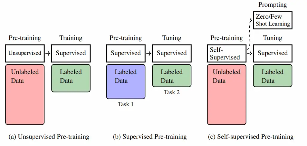
Figure 1.1 shows a comparison of the above three pre-training approaches. Self-supervised
pre-training is so successful that most current state-of-the-art NLP models are based on this
paradigm. Therefore, in this chapter and throughout this blog, we will focus on self-supervised
pre-training. We will show how sequence models are pre-trained via self-supervision and how the
pre-trained models are applied.

1.1.2 Adapting Pre-trained Models

As mentioned above, two major types of models are widely used in NLP pre-training.

• Sequence Encoding Models. Given a sequence of words or tokens, a sequence encoding
  model represents this sequence as either a real-valued vector or a sequence of vectors, and
  obtains a representation of the sequence. This representation is typically used as input to
  another model, such as a sentence classification system.

Fig. 1.1: Illustration of unsupervised, supervised, and self-supervised pre-training. In unsupervised pre-training, the pre-training is performed on large-scale unlabeled data. It can be viewed as a preliminary step to have a good starting point for the subsequent optimization process, though considerable effort is still required to further train the model with labeled data after pre-training. In supervised pre-training, the underlying assumption is that different (supervised) learning tasks are related. So we can first train the model on one task, and transfer the resulting model to another task with some training or tuning effort. In self-supervised pre-training, a model is pre-trained on large-scale unlabeled data via self-supervision. The model can be well trained in this way, and we can efficiently adapt it to new tasks through fine-tuning or prompting.

• Sequence Generation Models. In NLP, sequence generation generally refers to the problem of generating a sequence of tokens based on a given context. The term context has different meanings across applications. For example, it refers to the preceding tokens in language modeling, and refers to the source-language sequence in machine translation².
  We need different techniques for applying these models to downstream tasks after pre-training.
  Here we are interested in the following two methods.

1.1.2.1 Fine-tuning of Pre-trained Models

For sequence encoding pre-training, a common method of adapting pre-trained models is fine-tuning. Let \(\text{Encode}_\theta(\cdot)\) denote an encoder with parameters \(\theta\); for example, \(\text{Encode}_\theta(\cdot)\) can be a standard Transformer encoder. 1. Model Architecture Provided we have pre-trained this model in some way and obtained the optimal parameters \(\hat{\theta}\), we can employ it to model any sequence and generate the corresponding representation: \begin{equation} H = \text{Encode}_{\hat{\theta}}(x) \label{eq:encoder} \end{equation} where \(x\) is the input sequence \(\{x_0, x_1, \ldots, x_m\}\), and \(H\) is the output representation which is a sequence of real-valued vectors \(\{h_0, h_1, \ldots, h_m\}\). 1.1. Text Classification System Because the encoder does not work as a standalone NLP system, it is often integrated as a component into a bigger system. Consider, for example, a text classification problem:

We can build a text classification system by stacking a classifier on top of the encoder. Let \(\text{Classify}_\omega(\cdot)\) be a neural network with parameters \(\omega\). Then: \begin{equation} \text{Pr}_{\omega,\hat{\theta}}(\cdot|x) = \text{Classify}_\omega(H) = \text{Classify}_\omega(\text{Encode}_{\hat{\theta}}(x)) \label{eq:classifier} \end{equation} Here \(\text{Pr}_{\omega,\hat{\theta}}(\cdot|x)\) is a probability distribution over the label set \(\{\text{positive}, \text{negative}, \text{neutral}\}\). For brevity, we use \(F_{\omega,\hat{\theta}}(\cdot)\) to denote \(\text{Classify}_\omega(\text{Encode}_{\hat{\theta}}(\cdot))\). 2. Fine-tuning Process Because the model parameters \(\omega\) and \(\hat{\theta}\) are not optimized for the classification task, we must adapt them:

• We can train \(F_{\omega,\hat{\theta}}(\cdot)\) on a labeled dataset as a supervised learning task
• The outcome is optimized parameters \(\tilde{\omega}\) and \(\tilde{\theta}\)
• Alternatively, we can freeze \(\hat{\theta}\) and only optimize \(\omega\)

3. Example Application Once fine-tuned, we can classify new text. Consider this travel website comment:

I love the food here. It’s amazing!

After tokenization to \(x_{\text{new}}\), the model produces: \begin{equation} F_{\tilde{\omega},\tilde{\theta}}(x_{\text{new}}) = \begin{bmatrix} \text{Pr}(\text{positive}|x_{\text{new}}) & \text{Pr}(\text{negative}|x_{\text{new}}) & \text{Pr}(\text{neutral}|x_{\text{new}}) \end{bmatrix} \label{eq:prediction} \end{equation} The label with maximum probability (here positive) is selected. 4. Conclusion

• Fine-tuning uses less labeled data than pre-training
• Computationally efficient adaptation method
• Only requires slight parameter adjustments

For more details, see Section~sec:advanced (to be implemented).

1.1.2.2 Prompting of Pre-trained Models

Unlike sequence encoding models, sequence generation models are often employed independently
to address language generation problems, such as question answering and machine translation,
without the need for additional modules. It is therefore straightforward to fine-tune these models as complete systems on downstream tasks. For example, we can fine-tune a pre-trained encoderdecoder multilingual model on some bilingual data to improve its performance on a specific translation task.

Among various sequence generation models, a notable example is the large language models
trained on very large amounts of data. These language models are trained to simply predict the next
token given its preceding tokens. Although token prediction is such a simple task that it has long
been restricted to “language modeling” only, it has been found to enable the learning of the general
knowledge of languages by repeating the task a large number of times. The result is that the
pre-trained large language models exhibit remarkably good abilities in token prediction, making
it possible to transform numerous NLP problems into simple text generation problems through
prompting the large language models. For example, we can frame the above text classification
problem as a text generation task

I love the food here. It’s amazing! I’m_________

Here _________ indicates the word or phrase we want to predict (call it the completion). If the predicted
word is happy, or glad, or satisfied or a related positive word, we can classify the text as positive.
This example shows a simple prompting method in which we concatenate the input text with I’m
to form a prompt. Then, the completion helps decide which label is assigned to the original text.
Given the strong performance of language understanding and generation of large language
models, a prompt can instruct the models to perform more complex tasks. Here is a prompt where
we prompt the LLM to perform polarity classification with an instruction.

Assume that the polarity of a text is a label chosen from {positive, negative,
neutral}. Identify the polarity of the input.
Input: I love the food here. It’s amazing!
Polarity:____

The first two sentences are a description of the task. Input and Polarity are indicators of the input
and output, respectively. We expect the model to complete the text and at the same time give the
correct polarity label. By using instruction-based prompts, we can adapt large language models to
solve NLP problems without the need for additional training.

This example also demonstrates the zero-shot learning capability of large language models,
which can perform tasks that were not observed during the training phase. Another method for
enabling new capabilities in a neural network is few-shot learning. This is typically achieved
through in-context learning (ICT). More specifically, we add some samples that demonstrate how
an input corresponds to an output. These samples, known as demonstrations, are used to teach
large language models how to perform the task. Below is an example involving demonstrations

Assume that the polarity of a text is a label chosen from {positive, negative,
neutral}. Identify the polarity of the input.
Input: The traffic is terrible during rush hours, making it difficult to reach the
airport on time.
Polarity: Negative
Input: The weather here is wonderful.
Polarity: Positive
Input: I love the food here. It’s amazing!
Polarity:_____

Prompting and in-context learning play important roles in the recent rise of large language
models. We will discuss these issues more deeply in Chapter 3. However, it is worth noting
that while prompting is a powerful way to adapt large language models, some tuning efforts are
still needed to ensure the models can follow instructions accurately. Additionally, the fine-tuning
process is crucial for aligning the values of these models with human values. More detailed
discussions of fine-tuning can be found in Chapter 4.

Colab-Compatible Code: Tokenization + Next Word Prediction

Output discussion:

• Original text: The weather is
• Tokenized words: [‘The’, ‘Ġweather’, ‘Ġis’]
• Token IDs: tensor([[ 464, 6193, 318]])
• Predicted next word: getting

1.2 Self-supervised Pre-training Tasks

In this section, we consider self-supervised pre-training approaches for different neural architectures, including decoder-only, encoder-only, and encoder-decoder architectures. We restrict our
discussion to Transformers since they form the basis of most pre-trained models in NLP. However, pre-training is a broad concept, and so we just give a brief introduction to basic approaches
in order to make this section concise.

1.2.1 Decoder-only Pre-training

The decoder-only architecture has been widely used in developing language models . For example, we can use a Transformer decoder as a language model by simply removing cross-attention sub-layers from it. Such a model predicts the distribution of tokens at a position given its preceding tokens, and the output is the token with the maximum probability. The standard way to train this model, as in the language modeling problem, is to minimize a loss function over a collection of token sequences. Let $\text{Decoder}_\theta(\cdot)$ denote a decoder with parameters $\theta$. At each position $i$, the decoder generates a distribution over the next token based on its preceding tokens $\{x_0, \ldots, x_i\}$, denoted by: \begin{equation} \Pr_\theta(\cdot|x_0, \ldots, x_i) \quad \text{(or } p^\theta_{i+1} \text{ for short)} \end{equation} Suppose we have the gold-standard distribution at the same position, denoted by $p^{\text{gold}}_{i+1}$. For language modeling:

• $p^{\text{gold}}_{i+1}$ is typically a one-hot representation of the correct token
• We define a loss function $\mathcal{L}(p^\theta_{i+1}, p^{\text{gold}}_{i+1})$ to measure the difference between:
  • Model prediction $p^\theta_{i+1}$
  • True distribution $p^{\text{gold}}_{i+1}$

In natural language processing, the standard choice is the \textbf{log-scale cross-entropy loss}: \begin{equation} \mathcal{L}(p^\theta_{i+1}, p^{\text{gold}}_{i+1}) = -\sum_{w \in \mathcal{V}} p^{\text{gold}}_{i+1}(w) \log p^\theta_{i+1}(w) \end{equation} where $\mathcal{V}$ is the vocabulary. For one-hot $p^{\text{gold}}_{i+1}$ (where $p^{\text{gold}}_{i+1}(w^*) = 1$ for the correct token $w^*$ and 0 otherwise), this simplifies to: \begin{equation} \mathcal{L}(p^\theta_{i+1}, p^{\text{gold}}_{i+1}) = -\log p^\theta_{i+1}(w^*) \end{equation}

5. Sequence Loss Given a sequence of $m$ tokens $\{x_0, \ldots, x_m\}$, the loss on this sequence is the sum of the loss over the positions $\{0, \ldots, m-1\}$, given by:
\begin{equation}
\text{Loss}_\theta(x_0, \ldots, x_m) = \sum_{i=0}^{m-1} \mathcal{L}(p^\theta_{i+1}, p^{\text{gold}}_{i+1}) = \sum_{i=0}^{m-1} \text{LogCrossEntropy}(p^\theta_{i+1}, p^{\text{gold}}_{i+1})
\label{eq:seq_loss}
\end{equation}
where:

• $\text{LogCrossEntropy}(\cdot)$ is the log-scale cross-entropy function
  
• $p^{\text{gold}}_{i+1}$ is the one-hot representation of $x_{i+1}$
  

6. Dataset-Level Objective For a dataset $\mathcal{D}$ of sequences, the pre-training objective becomes:
\begin{equation}
\hat{\theta} = \underset{\theta}{\operatorname{arg\,min}} \sum_{x \in \mathcal{D}} \text{Loss}_\theta(x)
\label{eq:objective}
\end{equation}

7. Using the Trained Model With optimized parameters $\hat{\theta}$, the pre-trained language model $\text{Decoder}_{\hat{\theta}}(\cdot)$ can compute:

1.2.2 Encoder-only Pre-training

An $\operatorname{Encoder}_\theta(\cdot)$ is a function that maps a token sequence $\mathbf{x} = (x_0, \ldots, x_m)$ to a sequence of vectors $\mathbf{H} = (\mathbf{h}_0, \ldots, \mathbf{h}_m)$.

Training this model requires special consideration since we lack gold-standard data for evaluating the real-valued outputs. The standard approach involves:

• Combining the encoder with output layers
  
• Using easily obtainable supervision signals
  

The architecture shown in Figure~1 demonstrates this approach:
\begin{equation}
\label{eq:softmax-output}
\begin{bmatrix}
p^{W,\theta}_1 \\
\vdots \\
p^{W,\theta}_m
\end{bmatrix}
= \operatorname{Softmax}\bigl(W\cdot\operatorname{Encoder}_\theta(\mathbf{x})\bigr)
\end{equation}
When treating each $\mathbf{h}_i$ as a row vector, the full sequence becomes:
\begin{equation}
\mathbf{H} =
\begin{bmatrix}
\mathbf{h}_0 \\
\vdots \\
\mathbf{h}_m
\end{bmatrix}
\in \mathbb{R}^{(m+1)\times d}
\end{equation}

As established in Definition~, the encoder processes token sequences into vector representations. These are then transformed into probability distributions via Equation~\eqref{eq:softmax-output}, where:

• $W$ represents the output layer weights
  
• $\theta$ denotes the encoder parameters