What is SciPy?

SciPy is an interactive Python session used as a data-processing library that is made to compete with its rivalries such as MATLAB, Octave, R-Lab, etc. It has many user-friendly, efficient, and easy-to-use functions that help to solve problems like numerical integration, interpolation, optimization, linear algebra, and statistics. The benefit of using the SciPy library in Python while making ML models is that it makes a strong programming language available for developing fewer complex programs and applications.

Installation of SciPy

To install SciPy in your system, you can use Python package manager pip. Before proceeding, make sure that you have Python already installed in your system. Here’s the step to install Python in your system.

Step 1: Firstly, Open terminal and Command Prompt in your system.

Step 2: Run the installation Command to install SciPy in your system.

pip install scipy

Step 3: Pip will be download and install SciPy along with dependencies. This process will may take some time depends on internet connection.

Step 4: To verify installation, you need to import SciPy in a Python script or interactive shell.

import scipy
print(scipy.__version__)

Now the installation of SciPy is successfully completed.

How does Data Analysis work with SciPy?

Data Preparation

• Import the necessary libraries: import numpy as np and import scipy as sp.
• Load or generate your dataset using NumPy or pandas.

Exploratory Data Analysis (EDA)

• Use descriptive statistics from SciPy’s stats module to gain insights into the dataset.
• Calculate measures such as mean, median, standard deviation, skewness, kurtosis, etc.

Output:

Statistical Hypothesis Testing

Use SciPy’s stats module for various hypothesis tests such as t-tests, chi-square tests, ANOVA, etc.

# Example of a t-test

t_stat, p_value = stats.ttest_ind(group1, group2)

Regression Analysis

Utilize the linregress function for linear regression analysis.

# Linear regression

slope, intercept, r_value, p_value, std_err = stats.linregress(x, y)

Signal and Image Processing

• Use the scipy.signal module for signal processing operations.
• Explore scipy.ndimage for image processing.

from scipy import signal, ndimage

# Example of convolution using signal processing

result = signal.convolve2d(image, kernel, mode=’same’, boundary=’wrap’)

Optimization

Employ the optimization functions in SciPy to find optimal parameter values.

from scipy.optimize import minimize

# Define an objective function

def objective_function(x):

return x[0]**2 + x[1]**2

result = minimize(objective_function, [0, 0])

Import SciPy

Once SciPy is installed , you need to import the SciPy module(s)

Linear Algebra

Determinant of a Matrix

Output:

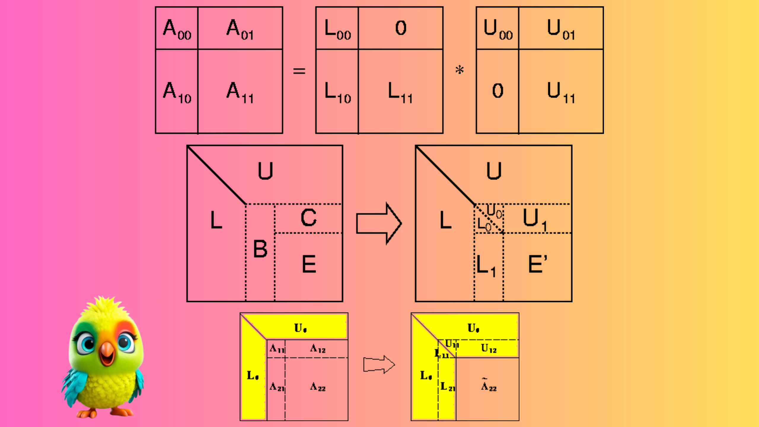
Compute pivoted LU decomposition of a Matrix

LU decomposition is a method that reduce matrix into constituent parts that helps in easier calculation of complex matrix operations. The decomposition methods are also called matrix factorization methods, are base of linear algebra in computers, even for basic operations such as solving systems of linear equations, calculating the inverse, and calculating the determinant of a matrix. The decomposition is: A = P L U where P is a permutation matrix, L lower triangular with unit diagonal elements, and U upper triangular.

Output:

Eigen values and Eigen vectors of this matrix

Output:

Solving systems of linear equations can also be done

Output:

Sparse Linear Algebra

SciPy has some routines for computing with sparse and potentially very large matrices. The necessary tools are in the submodule scipy.sparse.

Let’s look on how to construct a large sparse matrix

Output:

Linear Algebra for Sparse Matrices

Output:

Output:

There is a lot more that SciPy is capable of, such as Fourier Transforms, Bessel Functions, etc.

Subpackages in SciPy:

SciPy has a number of subpackages for various scientific computations which are shown in the following table:

However, for a detailed description, you can follow the official documentation.

These packages need to be imported exclusively prior to using them. For example:

Before looking at each of these functions in detail, let’s first take a look at the functions that are common both in NumPy and SciPy.

Basic Functions:

Interaction with NumPy:

SciPy builds on NumPy and therefore you can make use of NumPy functions itself to handle arrays. To know in-depth about these functions, you can simply make use of help(), info() or source() functions.

help():

To get information about any function, you can make use of the help() function. There are two ways in which this function can be used:

• without any parameters
• using parameters

Here is an example that shows both of the above methods:

When you execute the above code, the first help() returns the information about the cluster submodule. The second help() asks the user to enter the name of any module, keyword, etc for which the user desires to seek information. To stop the execution of this function, simply type ‘quit’ and hit enter.

info():

This function returns information about the desired functions, modules, etc.

source():

The source code is returned only for objects written in Python. This function does not return useful information in case the methods or objects are written in any other language such as C. However in case you want to make use of this function, you can do it as follows:

Special Functions:

SciPy provides a number of special functions that are used in mathematical physics such as elliptic, convenience functions, gamma, beta, etc. To look for all the functions, you can make use of help() function as described earlier.

Exponential and Trigonometric Functions:

SciPy’s Special Function package provides a number of functions through which you can find exponents and solve trigonometric problems.

Consider the following example:

EXAMPLE:

OUTPUT:

1000.0
8.0
1.0
0.7071067811865475

​There are many other functions present in the special functions package of SciPy that you can try for yourself.

Integration Functions:

SciPy provides a number of functions to solve integrals. Ranging from ordinary differential integrator to using trapezoidal rules to compute integrals, SciPy is a storehouse of functions to solve all types of integrals problems.

General Integration:

SiPy provides a function named quad to calculate the integral of a function which has one variable. The limits can be ( ) to indicate infinite limits. The syntax of the quad() function is as follows:

SYNTAX:

quad(func, a, b, args=(), full_output=0, epsabs=1.49e-08, epsrel=1.49e-08, limit=50, points=None, weight=None, wvar=None, wopts=None, maxp1=50, limlst=50)

Here, the function will be integrated between the limits a and b (can also be infinite).

EXAMPLE:

In the above example, the function ‘a’ is evaluated between the limits 0, 1. When this code is executed, you will see the following output.

OUTPUT:

(3.9086503371292665, 4.3394735994897923e-14)

Double Integral Function:

SciPy provides dblquad that can be used to calculate double integrals. A double integral, as many of us know, consists of two real variables. The dblquad() function will take the function to be integrated as its parameter along with 4 other variables which define the limits and the functions dy and dx.

EXAMPLE:

OUTPUT:

-1.3333333333333335, 1.4802973661668755e-14)

SciPy provides various other functions to evaluate triple integrals, n integrals, Romberg Integrals, etc that you can explore further in detail. To find all the details about the required functions, use the help function.

Optimization Functions:

The scipy.optimize provides a number of commonly used optimization algorithms which can be seen using the help function.

It basically consists of the following:

• Unconstrained and constrained minimization of multivariate scalar functions i.e minimize (eg. BFGS, Newton Conjugate Gradient, Nelder_mead simplex, etc)
• Global optimization routines (eg. differential_evolution, dual_annealing, etc)
• Least-squares minimization and curve fitting (eg. least_squares, curve_fit, etc)
• Scalar univariate functions minimizers and root finders (eg. minimize_scalar and root_scalar)
• Multivariate equation system solvers using algorithms such as hybrid Powell, Levenberg-Marquardt.

Rosenbrook Function:

Rosenbrook function ( rosen) is a test problem used for gradient-based optimization algorithms. It is defined as follows in SciPy:

EXAMPLE:

OUTPUT: 7371.0399999999945

Nelder-Mead:

The Nelder-Mead method is a numerical method often used to find the min/ max of a function in a multidimensional space. In the following example, the minimize method is used along with the Nelder-Mead algorithm.

EXAMPLE:

OUTPUT: array([0.96570182, 0.93255069, 0.86939478, 0.75497872, 0.56793357])

Interpolation Functions:

In the field of numerical analysis, interpolation refers to constructing new data points within a set of known data points. The SciPy library consists of a subpackage named scipy.interpolate that consists of spline functions and classes, one-dimensional and multi-dimensional (univariate and multivariate) interpolation classes, etc.

Univariate Interpolation:

Univariate interpolation is basically an area of curve-fitting which finds the curve that provides an exact fit to a series of two-dimensional data points. SciPy provides interp1d function that can be utilized to produce univariate interpolation.

EXAMPLE:

OUTPUT:

Multivariate Interpolation:

Multivariate interpolation (spatial interpolation ) is a kind interpolation on functions that consist of more than one variables. The following example demonstrates an example of the
Interpolating over a 2-D grid using the interp2d(x, y, z) function basically will use x, y, z arrays to approximate some function interp2d function. f: “z = f(x, y)” and returns a function whose call method uses spline interpolation to find the value of new points.
EXAMPLE:

OUTPUT:

Fourier Transform Functions:

Fourier analysis is a method that deals with expressing a function as a sum of periodic components and recovering the signal from those components. The fft functions can be used to return the discrete Fourier transform of a real or complex sequence.

EXAMPLE:

OUTPUT: [ 6.+0.j -2.+2.j -2.+0.j -2.-2.j ]

Similarly, you can find the inverse of this by using the ifft function as follows:

EXAMPLE:

OUTPUT: [ 1.5+0.j -0.5–0.5j -0.5+0.j -0.5+0.5j]

Signal Processing Functions:

Signal processing deals with analyzing, modifying and synthesizing signals such as sound, images, etc. SciPy provides some functions using which you can design, filter and interpolate one-dimensional and two-dimensional data.

Filtering:

By filtering a signal, you basically remove unwanted components from it. To perform ordered filtering, you can make use of the order_filter function. This function basically performs ordered filtering on an array. The syntax of this function is as follows:

SYNTAX:

order_filter(a, domain, rank)

a = N-dimensional input array

domain = mask array having the same number of dimensions as a

rank = Non-negative number that selects elements from the list after it has been sorted (0 is the smallest followed by 1…)

EXAMPLE:

OUTPUT:

[[ 0 1 2 3 4]
[ 5 6 7 8 9]
[10 11 12 13 14]
[15 16 17 18 19]
[20 21 22 23 24]
[25 26 27 28 29]
[30 31 32 33 34]]

[[ 0. 1. 2. 3. 0.]
[ 5. 6. 7. 8. 3.]
[10. 11. 12. 13. 8.]
[15. 16. 17. 18. 13.]
[20. 21. 22. 23. 18.]
[25. 26. 27. 28. 23.]
[ 0. 25. 26. 27. 28.]]

Waveforms:

The scipy.signal subpackage also consists of various functions that can be used to generate waveforms. One such function is chirp. This function is a frequency-swept cosine generator and the syntax is as follows:

SYNTAX:
chirp(t, f0, t1, f1, method=’linear’, phi=0, vertex_zero=True)

where,

OUTPUT:

Linear Algebra:

Linear algebra deals with linear equations and their representations using vector spaces and matrices. SciPy is built on ATLAS LAPACK and BLAS libraries and is extremely fast in solving problems related to linear algebra. In addition to all the functions from numpy.linalg, scipy.linalg also provides a number of other advanced functions. Also, if numpy.linalg is not used along with ATLAS LAPACK and BLAS support, scipy.linalg is faster than numpy.linalg.

Finding the Inverse of a Matrix:

Mathematically, the inverse of a matrix A is the matrix such that where is the identity matrix consisting of ones down the main diagonal denoted as B=A-1. In SciPy, this inverse can be obtained using the linalg.inv method.

EXAMPLE:

OUTPUT:

[[-0.6 0.4]
[ 0.8 -0.2]]

Finding the Determinants:

The value derived arithmetically from the coefficients of the matrix is known as the determinant of a square matrix. In SciPy, this can be done using a function det which has the following syntax:

SYNTAX:
det(a, overwrite_a=False, check_finite=True)
where,

a : (M, M) Is a square matrix

overwrite_a( bool, optional) : Allow overwriting data in a

check_finite ( bool, optional): To check whether the input matrix consists only of finite numbers

EXAMPLE:

OUTPUT: -5.0

Sparse Eigenvalues:

Eigenvalues are a specific set of scalars linked with linear equations. The ARPACK provides that allow you to find eigenvalues ( eigenvectors ) quite fast. The complete functionality of ARPACK is packed within two high-level interfaces which are scipy.sparse.linalg.eigs and scipy.sparse.linalg.eigsh. eigs. The eigs interface allows you to find the eigenvalues of real or complex nonsymmetric square matrices whereas the eigsh interface contains interfaces for real-symmetric or complex-hermitian matrices.

The eigh function solves a generalized eigenvalue problem for a complex Hermitian or real symmetric matrix.

EXAMPLE:

OUTPUT:

Selected eigenvalues : [-2.53382695 1.66735639 3.69488657 12.17158399]
Complex ndarray : [[ 0.69205614 0.5829305 0.25682823 -0.33954321]
[-0.68277875 0.46838936 0.03700454 -0.5595134 ]
[ 0.23275694 -0.29164622 -0.72710245 -0.57627139]
[ 0.02637572 -0.59644441 0.63560361 -0.48945525]]

Spatial Data Structures and Algorithms:

Spatial data basically consists of objects that are made up of lines, points, surfaces, etc. The scipy.spatial package of SciPy can compute Voronoi diagrams, triangulations, etc using the Qhull library. It also consists of KDTree implementations for nearest-neighbor point queries.

Delaunay triangulations:

Mathematically, Delaunay triangulations for a set of discrete points in a plane is a triangulation such that no point in the given set of points is inside the circumcircle of any triangle.

EXAMPLE:

OUTPUT:

Multidimensional Image Processing Functions:

Image processing basically deals with performing operations on an image to retrieve information or to get an enhanced image from the original one. The scipy.ndimage package consists of a number of image processing and analysis functions designed to work with arrays of arbitrary dimensionality.

Convolution and correlation:

SciPy provides a number of functions that allow correlation and convolution of images.

• The function correlate1d can be used to calculate one-dimensional correlation along a given axis
• The function correlate allows multidimensional correlation of any given array with the specified kernel
• The function convolve1d can be used to calculate one-dimensional convolution along a given axis
• The function convolve allows multidimensional convolution of any given array with the specified kernel

EXAMPLE:

OUTPUT: array([ 9, 13, 7, 15, 11, 14, 24, 17])

File IO:

The scipy.io package provides a number of functions that help you manage files of different formats such as MATLAB files, IDL files, Matrix Market files, etc.

To make use of this package, you will need to import it as follows:

For complete information on subpackage, you can refer to the official document on File IO.

SciPy is an extensive library that offers a wide variety of functions across many different scientific and mathematical domains. Below is a comprehensive list of the primary functions grouped by category. Note that this list will not cover every single function in SciPy but will give you a good overview of the key modules and their functions.

1. Optimization (scipy.optimize)

• scipy.optimize.minimize: Minimization of scalar or multi-variable functions.
• scipy.optimize.fmin: Simplex method to minimize scalar functions.
• scipy.optimize.fminbound: Minimization of a scalar function within bounds.
• scipy.optimize.linprog: Solves linear programming problems.
• scipy.optimize.least_squares: Solves nonlinear least-squares problems.
• scipy.optimize.root: Find the roots of a function.
• scipy.optimize.curve_fit: Fit a function to data using least squares.
• scipy.optimize.differential_evolution: Performs global optimization using differential evolution.
• scipy.optimize.brute: Performs a brute-force optimization search over a specified parameter grid.

2. Integration (scipy.integrate)

• scipy.integrate.quad: Adaptive quadrature for single integrals.
• scipy.integrate.dblquad: Adaptive quadrature for double integrals.
• scipy.integrate.tplquad: Adaptive quadrature for triple integrals.
• scipy.integrate.odeint: Integrates ordinary differential equations.
• scipy.integrate.simps: Simpson’s rule for numerical integration.
• scipy.integrate.trapz: Trapezoidal rule for numerical integration.
• scipy.integrate.fixed_quad: Fixed-order quadrature rule for integration.
• scipy.integrate.quadrature: Gauss-Kronrod quadrature for integration.

3. Linear Algebra (scipy.linalg)

• scipy.linalg.solve: Solve a system of linear equations.
• scipy.linalg.inv: Compute the inverse of a matrix.
• scipy.linalg.det: Compute the determinant of a matrix.
• scipy.linalg.eig: Compute the eigenvalues and eigenvectors of a matrix.
• scipy.linalg.svd: Compute the singular value decomposition (SVD) of a matrix.
• scipy.linalg.lu: LU decomposition of a matrix.
• scipy.linalg.qr: QR decomposition of a matrix.
• scipy.linalg.cholesky: Cholesky decomposition of a matrix.
• scipy.linalg.norm: Compute the matrix or vector norm.
• scipy.linalg.pinv: Compute the Moore-Penrose pseudoinverse of a matrix.

4. Interpolation (scipy.interpolate)

• scipy.interpolate.interp1d: Interpolate a 1-dimensional function.
• scipy.interpolate.interp2d: Interpolate a 2-dimensional function.
• scipy.interpolate.griddata: Interpolate scattered data in multiple dimensions.
• scipy.interpolate.CubicSpline: Spline interpolation for 1-dimensional data.
• scipy.interpolate.Rbf: Radial basis function interpolation.
• scipy.interpolate.BarycentricInterpolator: Barycentric Lagrange interpolation.
• scipy.interpolate.PchipInterpolator: Piecewise cubic Hermite interpolator.
• scipy.interpolate.KroghInterpolator: Interpolate using a polynomial fit.
• scipy.interpolate.Bessel: Bessel interpolation (for periodic data).

5. Statistics (scipy.stats)

• scipy.stats.describe: Return descriptive statistics of data.
• scipy.stats.mean: Compute the arithmetic mean of data.
• scipy.stats.variance: Compute the variance of data.
• scipy.stats.skew: Compute the skewness of data.
• scipy.stats.kurtosis: Compute the kurtosis of data.
• scipy.stats.ttest_ind: Independent t-test.
• scipy.stats.ttest_rel: Paired t-test.
• scipy.stats.ks_2samp: Kolmogorov-Smirnov test for two samples.
• scipy.stats.chisquare: Chi-squared test.
• scipy.stats.f_oneway: One-way ANOVA.
• scipy.stats.binom: Binomial distribution.
• scipy.stats.norm: Normal (Gaussian) distribution.
• scipy.stats.poisson: Poisson distribution.
• scipy.stats.gamma: Gamma distribution.
• scipy.stats.lognorm: Log-normal distribution.
• scipy.stats.expon: Exponential distribution.
• scipy.stats.mannwhitneyu: Mann-Whitney U test for comparing two independent samples.
• scipy.stats.spearmanr: Spearman’s rank correlation.

6. Signal Processing (scipy.signal)

• scipy.signal.convolve: Convolution of two signals.
• scipy.signal.correlate: Cross-correlation of two signals.
• scipy.signal.fftconvolve: Convolution using FFT.
• scipy.signal.butter: Design a Butterworth filter.
• scipy.signal.cheby1: Design a Chebyshev Type I filter.
• scipy.signal.cheby2: Design a Chebyshev Type II filter.
• scipy.signal.firwin: Design a Finite Impulse Response (FIR) filter.
• scipy.signal.sosfilt: Apply a second-order section (SOS) filter.
• scipy.signal.find_peaks: Find peaks in data.
• scipy.signal.cwt: Continuous wavelet transform.
• scipy.signal.resample: Resample data using Fourier method.
• scipy.signal.decimate: Apply a decimation filter to down-sample a signal.

7. Multidimensional Image Processing (scipy.ndimage)

• scipy.ndimage.convolve: Convolution of multi-dimensional arrays.
• scipy.ndimage.zoom: Zoom into multi-dimensional arrays.
• scipy.ndimage.gaussian_filter: Apply Gaussian filter to multi-dimensional arrays.
• scipy.ndimage.binary_dilation: Binary dilation operation.
• scipy.ndimage.binary_erosion: Binary erosion operation.
• scipy.ndimage.label: Label connected components in an array.
• scipy.ndimage.distance_transform_edt: Compute the Euclidean distance transform.
• scipy.ndimage.sobel: Compute the Sobel filter for edge detection.
• scipy.ndimage.median_filter: Apply median filter to multi-dimensional data.

8. Sparse Matrices (scipy.sparse)

• scipy.sparse.csr_matrix: Compressed sparse row matrix format.
• scipy.sparse.csc_matrix: Compressed sparse column matrix format.
• scipy.sparse.dok_matrix: Dictionary of keys sparse matrix format.
• scipy.sparse.lil_matrix: List of lists sparse matrix format.
• scipy.sparse.eye: Create a sparse identity matrix.
• scipy.sparse.random: Generate sparse random matrices.

9. File I/O (scipy.io)

• scipy.io.loadmat: Load MATLAB .mat file.
• scipy.io.savemat: Save data to MATLAB .mat file.
• scipy.io.mmread: Read Matrix Market format data.
• scipy.io.mmwrite: Write Matrix Market format data.
• scipy.io.wavfile.read: Read a WAV file.
• scipy.io.wavfile.write: Write to a WAV file.

10. Special Functions (scipy.special)

• scipy.special.gamma: Gamma function.
• scipy.special.besselj: Bessel function of the first kind.
• scipy.special.ellipe: Complete elliptic integral of the second kind.
• scipy.special.erf: Error function.
• scipy.special.factorial: Factorial of a number.
• scipy.special.lambertw: Lambert W function.
• scipy.special.sph_jn: Spherical Bessel function of the first kind.

11. Cluster Analysis (scipy.cluster)

• scipy.cluster.hierarchy.linkage: Perform hierarchical/agglomerative clustering.
• scipy.cluster.hierarchy.dendrogram: Plot a dendrogram.
• scipy.cluster.vq.kmeans: Perform k-means clustering.
• scipy.cluster.vq.vq: Quantize data to a codebook (vector quantization).

12. Polynomial Functions (scipy.poly)

• scipy.polyfit: Polynomial curve fitting.
• scipy.polyval: Evaluate a polynomial at specified values.
• scipy.polynomial.Polynomial: Class for working with polynomials.

Conclusion

SciPy is an extensive library, and this list includes many of its core functions. Its rich functionality spans optimization, integration, linear algebra, interpolation, statistics, signal processing, image processing, sparse matrices, special functions, and more. These functions are indispensable for solving real-world scientific and mathematical problems, making SciPy a powerful tool for engineers, scientists, data analysts, and machine learning practitioners.