


 and How Data Passes Through Them")


, and Neural Networks in a structured way")
")


What is a Confusion Matrix?
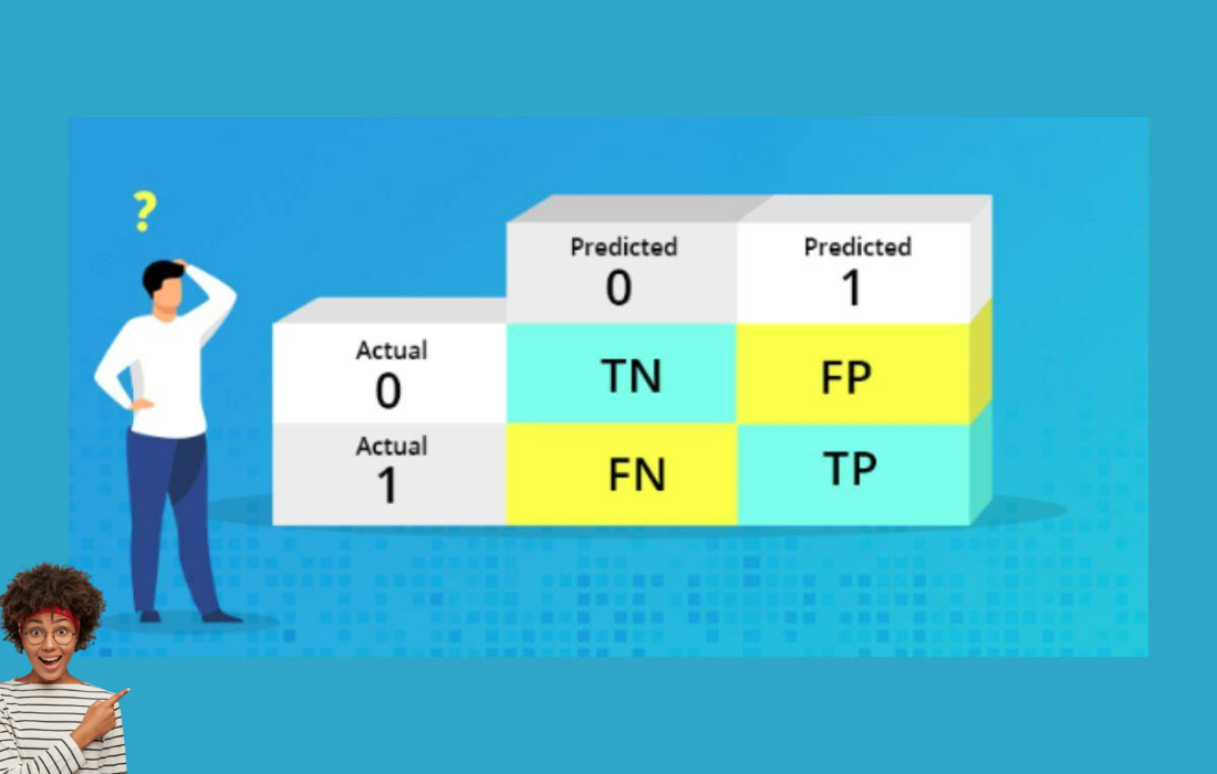
In machine learning, particularly in the field of classification, the confusion matrix is a useful tool for evaluating the performance of a binary classifier. It is a 2×2 table that helps to understand the accuracy of a classifier by comparing the predicted labels with the actual labels. The confusion matrix provides insight into how well a model is classifying the data and where it’s making errors.
The confusion matrix breaks down the predictions into four key categories:
| Actual\Predicted | Positive (Predict +) | Negative (Predict -) |
|---|---|---|
| Positive (Actual +) | True Positive (TP) | False Negative (FN) |
| Negative (Actual -) | False Positive (FP) | True Negative (TN) |
Let’s look at each of these terms in detail:
- True Positive (TP): The number of positive samples correctly predicted as positive.
- False Positive (FP): The number of negative samples incorrectly predicted as positive.
- True Negative (TN): The number of negative samples correctly predicted as negative.
- False Negative (FN): The number of positive samples incorrectly predicted as negative.
These terms allow us to derive several key performance metrics for evaluating the classifier’s accuracy.
Key Metrics Derived from the Confusion Matrix
The confusion matrix enables the calculation of several important metrics that help assess the performance of a binary classification model. Here are the most commonly used metrics:
1. Accuracy
Accuracy represents the overall correctness of the model, calculated as the percentage of correct predictions out of all predictions.
\[
\text{Accuracy} = \frac{TP + TN}{TP + TN + FP + FN}
\]
2. Precision
Precision is the percentage of true positive predictions out of all positive predictions made by the model. It answers the question: “Of all the samples predicted as positive, how many were actually positive?”
\[
\text{Precision} = \frac{\text{TP}}{\text{TP} + \text{FP}}
\]
3. Recall (Sensitivity)
Recall is the percentage of true positive predictions out of all actual positive instances. It tells us how well the model is identifying positive samples.
\[
\text{Recall} = \frac{TP}{TP + FN}
\]
4. F1-Score
The F1-Score is the harmonic mean of precision and recall, providing a single metric that balances both concerns. It’s especially useful when the class distribution is imbalanced.
\[
\text{F1-Score} = 2 \times \frac{\text{Precision} \times \text{Recall}}{\text{Precision} + \text{Recall}}
\]
5. Specificity
Specificity measures the proportion of actual negatives that are correctly identified by the model.
\[
\text{Specificity} = \frac{TN}{TN + FP}
\]
6. False Positive Rate (FPR)
FPR is the proportion of actual negatives that were incorrectly predicted as positives. It is the complement of specificity.
\[
\text{FPR} = \frac{FP}{TN + FP}
\]
Interpreting the Confusion Matrix
The confusion matrix helps assess how a model is performing in a detailed manner, especially in scenarios where accuracy alone is not enough. For instance:
- High Precision indicates that the model is making fewer false positive errors, which is crucial in applications like email spam filtering, where predicting a legitimate email as spam (false positive) could have serious consequences.
- High Recall indicates that the model is correctly identifying most of the actual positive instances, which is important in fields like medical diagnostics where missing a positive case (false negative) can be critical.
- F1-Score is used when you need a balance between precision and recall, and is especially useful when there’s an imbalance in the class distribution (e.g., fraud detection, where fraudulent transactions are much less common than non-fraudulent ones).
Example of a Confusion Matrix
Let’s say we have a model that predicts whether a person has a disease based on some features. After applying the model to a test dataset, the confusion matrix looks like this:
| Actual\Predicted | Positive (Predict +) | Negative (Predict -) |
|---|---|---|
| Positive (Actual +) | 80 (TP) | 20 (FN) |
| Negative (Actual -) | 30 (FP) | 70 (TN) |
From this confusion matrix, we can calculate:
Let’s break down the calculations you provided for Accuracy, Precision, Recall, and F1-Score and format them properly in LaTeX:
Given:
- True Positives (TP) = 80
- True Negatives (TN) = 70
- False Positives (FP) = 30
- False Negatives (FN) = 20
1. Accuracy
The formula for Accuracy is:
\[
\text{Accuracy} = \frac{TP + TN}{TP + TN + FP + FN}
\]
Substituting in the values:
\[
\text{Accuracy} = \frac{80 + 70}{80 + 70 + 30 + 20} = \frac{150}{200} = 0.75 \quad (75% \text{ accuracy})
\]
2. Precision
The formula for Precision is:
\[
\text{Precision} = \frac{TP}{TP + FP}
\]
Substituting in the values:
\[
\text{Precision} = \frac{80}{80 + 30} = \frac{80}{110} \approx 0.727 \quad (72.7% \text{ precision})
\]
3. Recall
The formula for Recall is:
\[
\text{Recall} = \frac{TP}{TP + FN}
\]
Substituting in the values:
\[
\text{Recall} = \frac{80}{80 + 20} = \frac{80}{100} = 0.8 \quad (80% \text{ recall})
\]
4. F1-Score
The formula for the F1-Score is:
\[
\text{F1-Score} = 2 \times \frac{\text{Precision} \times \text{Recall}}{\text{Precision} + \text{Recall}}
\]
Substituting in the calculated Precision and Recall values:
\[
\text{F1-Score} = 2 \times \frac{0.727 \times 0.8}{0.727 + 0.8} = 2 \times \frac{0.5816}{1.527} \approx 0.762 \quad (76.2% \text{ F1-score})
\]
This concludes your set of calculations formatted clearly. If you need further clarification or additional calculations, feel free to ask!
Conclusion
The confusion matrix is a powerful tool for evaluating a binary classifier’s performance. It provides insight into how well the model is classifying data and allows you to compute a variety of performance metrics like accuracy, precision, recall, and F1-score. Understanding these metrics is essential for diagnosing issues with your classifier, such as whether it’s overfitting, underfitting, or making biased predictions. By leveraging the confusion matrix and its derived metrics, you can fine-tune your models to achieve the best performance possible for your use case.