


 and How Data Passes Through Them")


, and Neural Networks in a structured way")
")

 That You’ll Want to Buy for yourself")


Welcome to our mathematically rigorous exploration of tensors. This guide provides precise definitions, theoretical foundations, and worked examples ranging from elementary to advanced levels. All concepts are presented using proper mathematical notation with no reliance on programming languages.
The Story of Tensors: From Curved Surfaces to Cosmic Equations
Long ago, in the 19th century, a brilliant mathematician named Carl Friedrich Gauss was curious about the shape of the Earth. While studying curved surfaces like hills and valleys, he realized he needed a way to describe how things bend and stretch – not just on flat paper, but on real, bumpy surfaces. He planted the seeds for what would one day be known as tensor thinking, even though he didn’t call it that yet.
Years later, his student Bernhard Riemann took the idea further. Riemann dreamed of spaces that curved not just in two or three dimensions, but in many. He imagined weird, warping geometries where distances and angles changed – perfect for describing the universe itself. But he needed a new language to describe all this – a language of multi-dimensional quantities. The world wasn’t quite ready for it yet.
Then came Gregorio Ricci-Curbastro and his student Tullio Levi-Civita. These two Italian mathematicians quietly built the formal rules of this new language, which they called “absolute differential calculus” – what we now call tensor calculus. It was elegant, powerful… and completely ignored by most of the scientific world. It was just too abstract, too strange.
Until – in 1915 – Albert Einstein came knocking.
Einstein had a bold idea: gravity wasn’t a force pulling things together, but a result of space and time bending around mass. But how could he write equations for something so mind-bending?
Enter tensors.
With Ricci and Levi-Civita’s tools, Einstein was finally able to describe how planets orbit the sun, how light curves around stars, and how the universe itself expands – all in the language of tensors. The world paid attention.
Fast forward to today: if you’re building AI models, simulating black holes, or analyzing MRI scans, you’re using tensors. What once was an obscure, difficult idea has become the backbone of modern physics and machine learning.
Tensors started with geometry, found their destiny in Einstein’s relativity, and now live on in every deep learning model.
Tensors are fundamental mathematical objects that generalize scalars, vectors, and matrices to higher dimensions. They play a crucial role in physics, machine learning, and deep learning. In this blog, we’ll explore tensors with mathematical examples – one simple and one complex per subtopic-to solidify your understanding.
The History and Origin of Tensors From Mathematics to Modern AI
1. Early Foundations: Vector Calculus (1800s)
Key Developments
The mathematical precursors to tensors emerged in the 19th century:
\begin{align*}
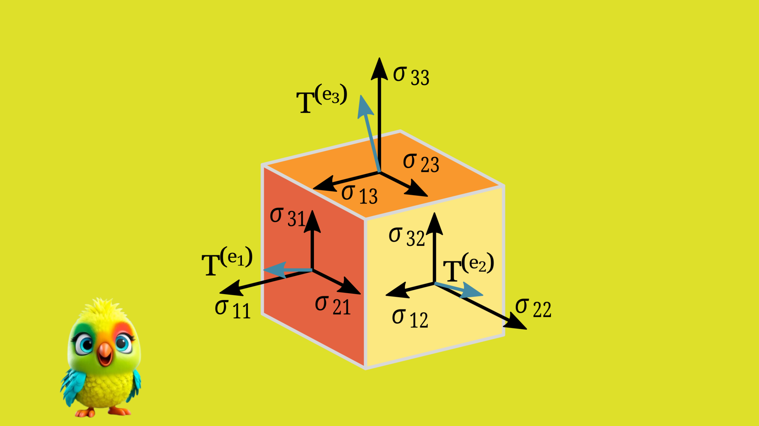
\text{Stress tensor in elasticity: } & \sigma_{ij} = \begin{bmatrix}
\sigma_{11} & \sigma_{12} \\
\sigma_{21} & \sigma_{22}
\end{bmatrix} \\
\text{Quaternion product: } & \mathbf{q} = a + b\mathbf{i} + c\mathbf{j} + d\mathbf{k}
\end{align*}
2. Formalization by Ricci and Levi-Civita (1890-1900)
The absolute differential calculus was developed with key notation:
\begin{equation*}
\text{Covariant derivative: } \nabla_k T^{ij} = \partial_k T^{ij} + \Gamma^{i}_{kl}T^{lj} + \Gamma^{j}_{kl}T^{il}
\end{equation*}
where $\Gamma^{i}_{jk}$ are Christoffel symbols.
3. Einstein’s General Relativity (1915)
The field equations demonstrate tensor power:
\begin{equation*}
G_{\mu\nu} = \frac{8\pi G}{c^4}T_{\mu\nu}
\end{equation*}
where:
\begin{align*}
G_{\mu\nu} & = R_{\mu\nu} – \frac{1}{2}Rg_{\mu\nu} \quad \text{(Einstein tensor)} \\
R_{\mu\nu} & \quad \text{(Ricci curvature tensor)} \\
g_{\mu\nu} & \quad \text{(Metric tensor)}
\end{align*}
4. Quantum Mechanics (1920s-1950s)
Tensor applications expanded:
\begin{equation*}
\text{Spin state: } |\psi\rangle = \alpha|\uparrow\rangle + \beta|\downarrow\rangle \quad \text{where } |\alpha|^2 + |\beta|^2 = 1
\end{equation*}
Moment of inertia tensor:
\begin{equation*}
I_{ij} = \int_V \rho(\mathbf{r})(r^2\delta_{ij} – r_ir_j) dV
\end{equation*}
5. Modern Computing and AI
Neural networks employ tensor operations:
\begin{equation*}
\text{Attention weights: } \mathbf{A} \in \mathbb{R}^{B \times H \times S \times S}
\end{equation*}
where:
- $B$ = batch size
- $H$ = number of attention heads
- $S$ = sequence length
Conclusion: Why Tensors Prevailed?
\begin{equation*}
\boxed{
\begin{aligned}
\text{Generality} & : \text{Unifies scalars, vectors, matrices} \\
\text{Physical fidelity} & : \text{Accurate in curved spacetime} \\
\text{Computational power} & : \text{Scalable to high dimensions}
\end{aligned}
}
\end{equation*}
1. Fundamentals of Tensors
Definition
A tensor of rank (order) r is a multilinear map:
\[
T : V_1^* \times V_2^* \times \cdots \times V_r^* \rightarrow \mathbb{R}
\]
where \( V_i^* \) are dual vector spaces.
Examples
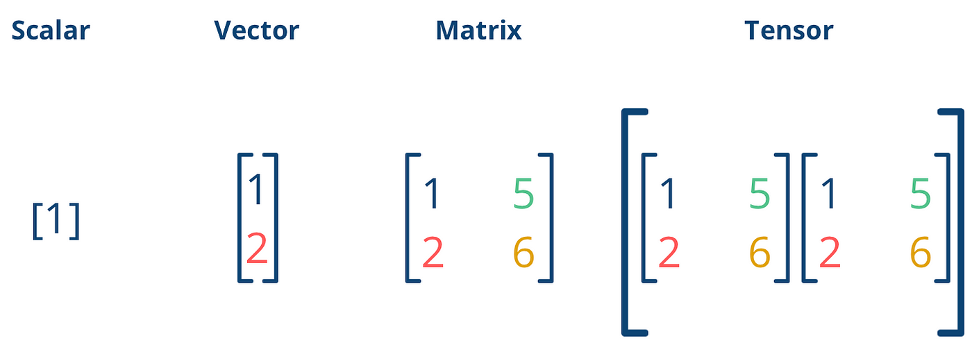
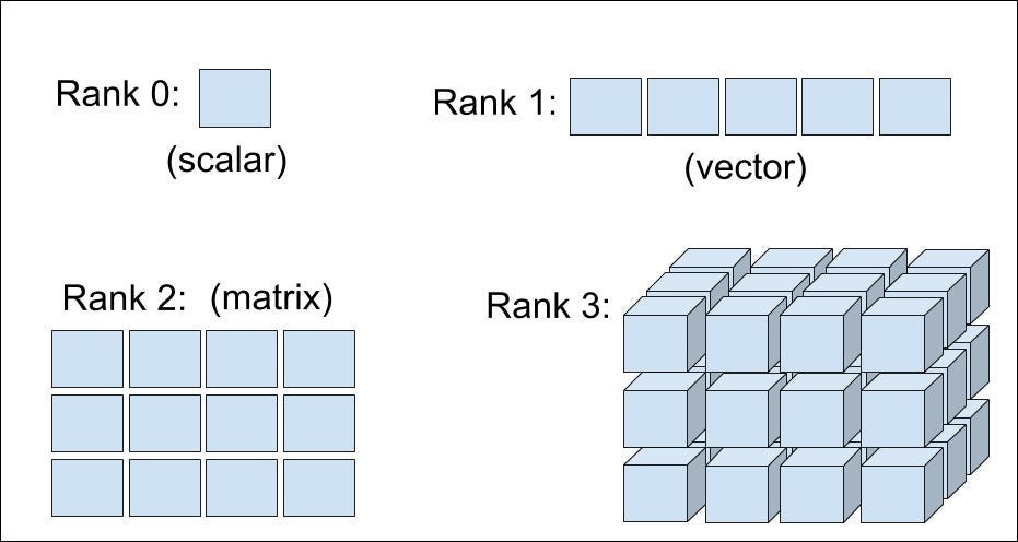
Rank-0 (Scalar):
– Temperature field: \( \phi(\mathbf{x}) = 25.0 \, \text{°C} \)
Rank-1 (Vector):
– Velocity field: \( \mathbf{v} = \begin{bmatrix} v_1 \\ v_2 \\ v_3 \end{bmatrix} \)
Rank-2 (Matrix):
– Stress tensor: \( \sigma = \begin{bmatrix} \sigma_{11} & \sigma_{12} \\ \sigma_{21} & \sigma_{22} \end{bmatrix} \)
Rank-3 (Advanced):
– Piezoelectric tensor: \( d_{ijk} \) relating strain to polarization
2. Tensor Algebra
Addition & Scalar Multiplication
Example 1 (Simple):
Let \( A, B \in \mathbb{R}^{2 \times 2} \):
\[
A = \begin{bmatrix} 1 & 2 \\ 3 & 4 \end{bmatrix}, \quad B = \begin{bmatrix} 5 & 6 \\ 7 & 8 \end{bmatrix}
\]
\[
A + B = \begin{bmatrix} 6 & 8 \\ 10 & 12 \end{bmatrix}, \quad 3A = \begin{bmatrix} 3 & 6 \\ 9 & 12 \end{bmatrix}
\]
Example 2 (Advanced):
For \( \mathbf{u}, \mathbf{v} \in \mathbb{R}^3 \):
\[
\mathbf{u} \otimes \mathbf{v} = \begin{bmatrix} u_1v_1 & u_1v_2 & u_1v_3 \\ u_2v_1 & u_2v_2 & u_2v_3 \\ u_3v_1 & u_3v_2 & u_3v_3 \end{bmatrix}
\]
3. Tensor Contraction
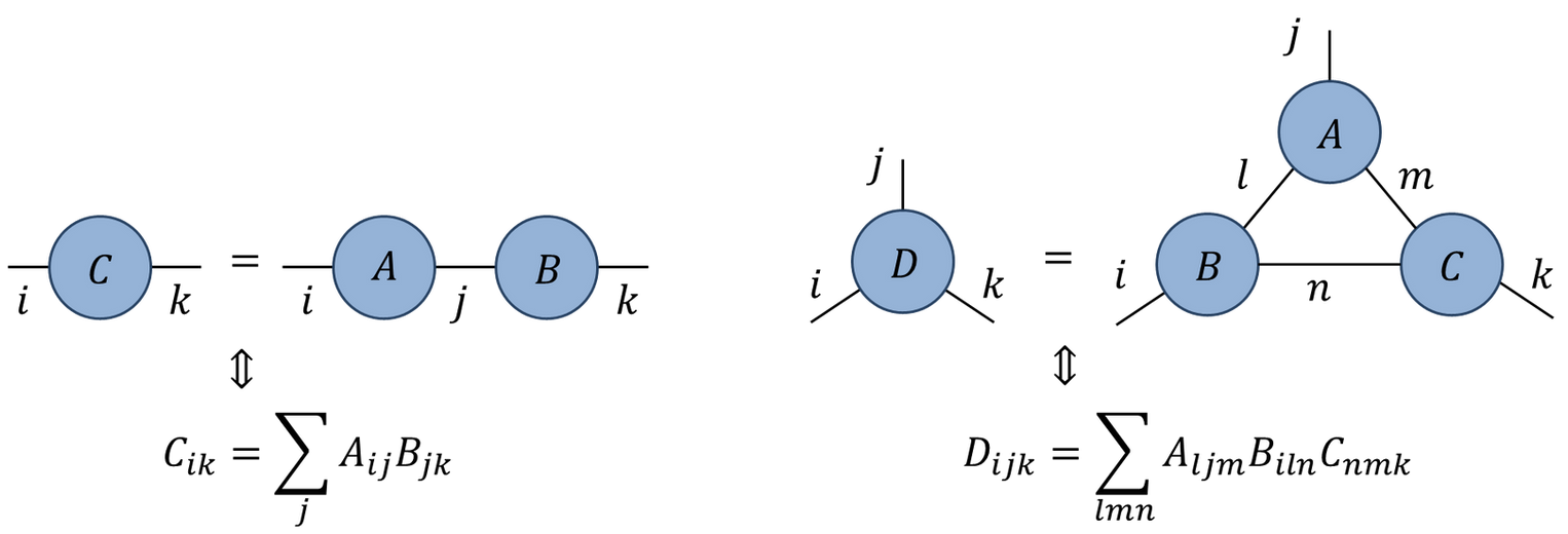
Definition
Given \( T^{i_1 \cdots i_p}_{j_1 \cdots j_q} \), contraction sums over paired indices:
\[
T^{ik}_{kj} \rightarrow S^i_j
\]

Example 1 (Simple): Matrix Trace
\[
\text{tr}(A) = A^i_i = \sum_{i=1}^n A_{ii}
\]
Example 2 (Advanced): General Relativity
Ricci curvature tensor from Riemann tensor:
\[
R_{μν} = R^λ_{μλν}
\]
4. Tensor Products

Outer Product
For \( \mathbf{u} \in \mathbb{R}^m \), \( \mathbf{v} \in \mathbb{R}^n \):
\[
\mathbf{u} \otimes \mathbf{v} = \mathbf{u} \mathbf{v}^\top
\]
Example:
\[
\begin{bmatrix} 1 \\ 2 \end{bmatrix} \otimes \begin{bmatrix} 3 & 4 \end{bmatrix} = \begin{bmatrix} 3 & 4 \\ 6 & 8 \end{bmatrix}
\]
Kronecker Product (Advanced)
For matrices \( A \in \mathbb{R}^{m×n} \), \( B \in \mathbb{R}^{p×q} \):
\[
A \otimes B = \begin{bmatrix} a_{11}B & \cdots & a_{1n}B \\ \vdots & \ddots & \vdots \\ a_{m1}B & \cdots & a_{mn}B \end{bmatrix}
\]
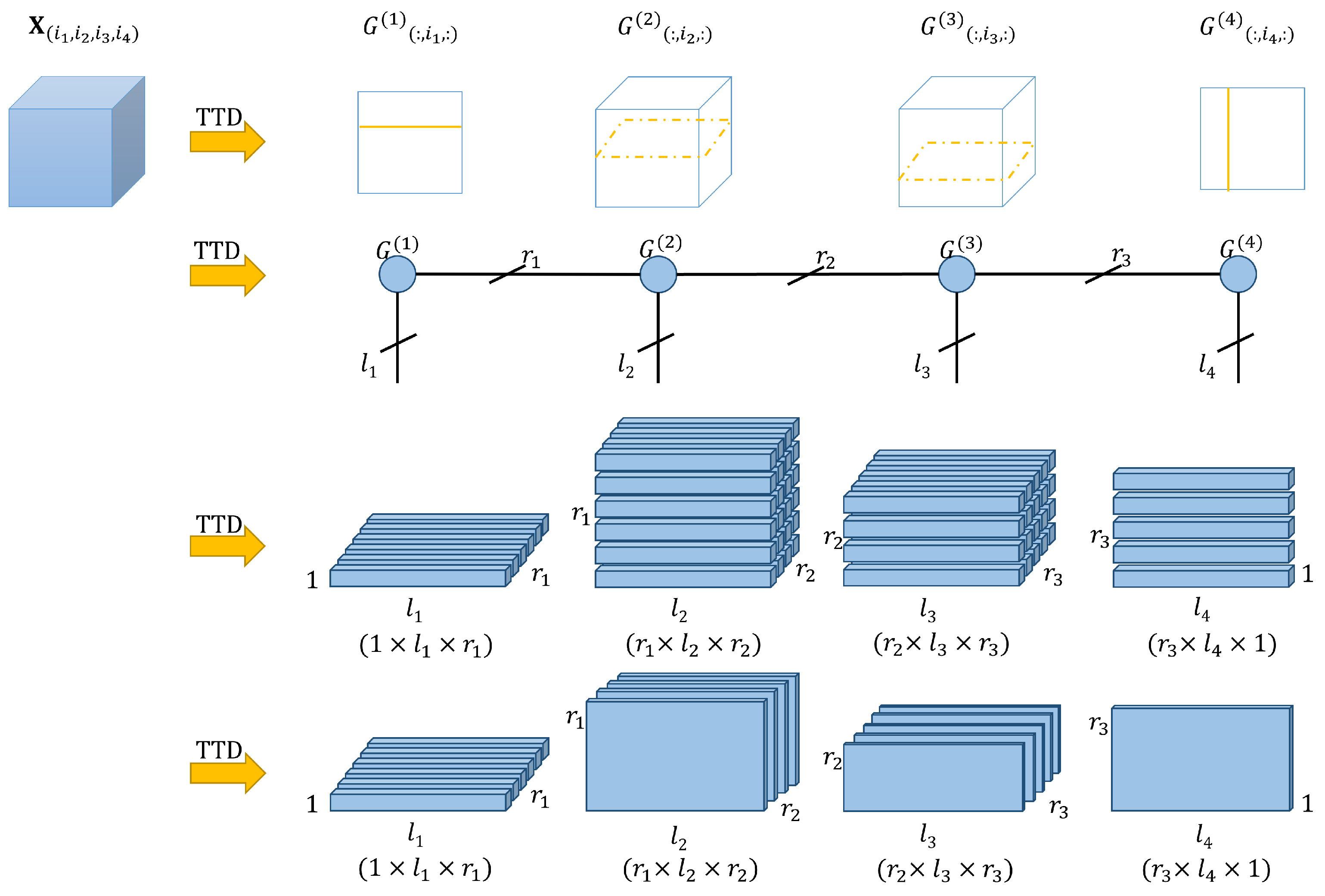
5. Tensor Decomposition
CP Decomposition
\[
\mathcal{T} \approx \sum_{r=1}^R \mathbf{a}_r \otimes \mathbf{b}_r \otimes \mathbf{c}_r
\]
Example (Simple):
A rank-1 approximation of a matrix:
\[
\begin{bmatrix} 2 & 4 \\ 3 & 6 \end{bmatrix} \approx \begin{bmatrix} 1 \\ 1.5 \end{bmatrix} \otimes \begin{bmatrix} 2 & 4 \end{bmatrix}
\]
Tucker Decomposition (Advanced)
\[
\mathcal{T} = \mathcal{G} \times_1 U \times_2 V \times_3 W
\]
where \( \mathcal{G} \) is the core tensor.
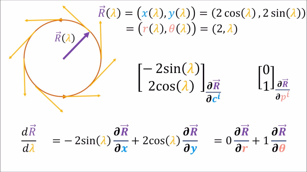
6. Covariant & Contravariant Tensors
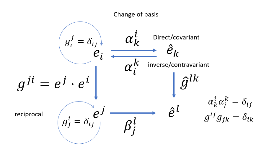
Transformation Laws
– Contravariant: \( T^{i’} = \frac{\partial x^{i’}}{\partial x^j} T^j \)
– Covariant: \( T_{i’} = \frac{\partial x^j}{\partial x^{i’}} T_j \)
Example (Advanced): Metric Tensor
In spherical coordinates:
\[
g_{μν} = \text{diag}(1, r^2, r^2 \sin^2 θ)
\]
7. Tensor Calculus
Gradient of Tensor Field
For \( \mathbf{T}(\mathbf{x}) \):
\[
(\nabla \mathbf{T})_{ijk} = \frac{\partial T_{ij}}{\partial x_k}
\]
Example (Advanced): Navier-Stokes Equations
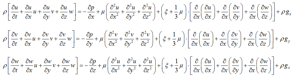
Stress tensor divergence:
\[
\nabla \cdot \sigma = \frac{\partial \sigma_{ij}}{\partial x_j}
\]
Conclusion
This mathematical treatment demonstrates how tensors:
1. Generalize scalars/vectors/matrices
2. Obey precise transformation rules
3. Enable modeling of complex physical systems