Partial Differential Equations (PDEs), Their Canonical Forms wave, heat, and Laplace equations

Partial differential equations (PDEs) are classified into different types based on their characteristics, which determine the nature of their solutions and the appropriate solution methods. The three most important PDEs in mathematical physics are:

Partial differential equations (PDEs) are used in machine learning (ML)—especially in advanced fields like:

Physics-informed neural networks (PINNs): These use PDEs to embed physical laws directly into the learning process (e.g., modeling fluid flow, heat transfer).
Computer vision: PDEs help with edge detection, image smoothing, and segmentation (e.g., Perona-Malik diffusion).
Optimization and training dynamics: Some training behaviors in neural networks are modeled using PDEs, especially when analyzing gradient flows.
Generative models: PDEs are used in score-based generative models (e.g., diffusion models), where the generation process solves a reverse-time stochastic differential equation.
Graph neural networks and manifold learning: PDEs model diffusion on graphs and geometric domains.

PDEs bridge physics, geometry, and ML to model continuous processes in a learnable way.

1. Physics-Informed Neural Networks (PINNs)

import torch
import torch.nn as nn

# Define the neural network
class PINN(nn.Module):
    def __init__(self):
        super().__init__()
        self.fc = nn.Sequential(
            nn.Linear(2, 20), nn.Tanh(),  # Input: (x, t)
            nn.Linear(20, 20), nn.Tanh(),
            nn.Linear(20, 1)              # Output: u(x,t)
        )
    
    def forward(self, x, t):
        return self.fc(torch.cat([x, t], dim=1))

# Loss function
def pde_loss(u, x, t, alpha=0.1):
    u_x = torch.autograd.grad(u.sum(), x, create_graph=True)[0]
    u_xx = torch.autograd.grad(u_x.sum(), x, create_graph=True)[0]
    u_t = torch.autograd.grad(u.sum(), t, create_graph=True)[0]
    return (u_t - alpha * u_xx).pow(2).mean()

# Training loop
model = PINN()
optimizer = torch.optim.Adam(model.parameters(), lr=1e-3)
for epoch in range(1000):
    x = torch.rand(100, 1, requires_grad=True)
    t = torch.rand(100, 1, requires_grad=True)
    u_pred = model(x, t)
    loss = pde_loss(u_pred, x, t)
    optimizer.zero_grad()
    loss.backward()
    optimizer.step()

import torch

import torch.nn as nn

# Define the neural network

class PINN(nn.Module):

def __init__(self):

super().__init__()

self.fc = nn.Sequential(

nn.Linear(2, 20), nn.Tanh(), # Input: (x, t)

nn.Linear(20, 20), nn.Tanh(),

nn.Linear(20, 1) # Output: u(x,t)

)

def forward(self, x, t):

return self.fc(torch.cat([x, t], dim=1))

# Loss function

def pde_loss(u, x, t, alpha=0.1):

u_x = torch.autograd.grad(u.sum(), x, create_graph=True)[0]

u_xx = torch.autograd.grad(u_x.sum(), x, create_graph=True)[0]

u_t = torch.autograd.grad(u.sum(), t, create_graph=True)[0]

return (u_t - alpha * u_xx).pow(2).mean()

# Training loop

model = PINN()

optimizer = torch.optim.Adam(model.parameters(), lr=1e-3)

for epoch in range(1000):

x = torch.rand(100, 1, requires_grad=True)

t = torch.rand(100, 1, requires_grad=True)

u_pred = model(x, t)

loss = pde_loss(u_pred, x, t)

optimizer.zero_grad()

loss.backward()

optimizer.step()

PDE Example: Navier-Stokes Equations (Fluid Flow)
PDE:
$$
\frac{\partial \mathbf{u}}{\partial t} + (\mathbf{u} \cdot \nabla) \mathbf{u} = -\nabla p + \nu \nabla^2 \mathbf{u}, \quad \nabla \cdot \mathbf{u} = 0
$$
PINN Implementation:
A neural network $ \mathbf{u}_\theta(x,t) $ is trained to satisfy:
– The PDE residual:
$$
\mathcal{L}_{\text{PDE}} = \left\| \frac{\partial \mathbf{u}_\theta}{\partial t} + (\mathbf{u}_\theta \cdot \nabla) \mathbf{u}_\theta + \nabla p_\theta – \nu \nabla^2 \mathbf{u}_\theta \right\|^2
$$
– Boundary/initial conditions:
$$
\mathcal{L}_{\text{BC}} = \left\| \mathbf{u}_\theta(x,t) – \mathbf{u}_{\text{true}}(x,t) \right\|^2_{\partial \Omega}
$$
Loss Function:
$$
\mathcal{L} = \mathcal{L}_{\text{PDE}} + \mathcal{L}_{\text{BC}}
$$

2. Computer Vision (Perona-Malik Diffusion)

import numpy as np

from scipy.ndimage import laplace

def perona_malik_diffusion(image, iterations=10, k=0.1):

img = image.copy()

for _ in range(iterations):

grad = np.gradient(img)

grad_norm = np.sqrt(grad[0]**2 + grad[1]**2)

g = 1 / (1 + (grad_norm / k)**2) # Diffusivity

img += 0.1 * laplace(g * grad[0]) + 0.1 * laplace(g * grad[1])

return img

# Example usage

noisy_image = np.random.randn(64, 64)

denoised = perona_malik_diffusion(noisy_image)

PDE Example: Nonlinear Diffusion for Image Denoising
PDE:
$$
\frac{\partial I}{\partial t} = \nabla \cdot \left( g(|\nabla I|) \nabla I \right), \quad g(|\nabla I|) = \frac{1}{1 + (|\nabla I|/k)^2}
$$
Role:
– $ I(x,y,t) $: Image intensity.
– $ g(|\nabla I|) $: Edge-preserving diffusivity.
– Effect: Smooths homogeneous regions while preserving edges.

3. Optimization (Gradient Flow PDEs)

import jax

import jax.numpy as jnp

def loss(theta):

return theta ** 4

grad_flow = jax.jit(jax.grad(loss))

theta = 2.0 # Initial parameter

lr = 0.01

for step in range(100):

theta -= lr * grad_flow(theta) # PDE: dθ/dt = -∇L(θ)

PDE Example: Heat Equation as Gradient Descent
PDE:
$$
\frac{\partial \theta}{\partial t} = -\nabla_\theta \mathcal{L}(\theta)
$$
Interpretation:
– $ \theta(t) $: Neural network parameters.
– $ \mathcal{L}(\theta) $: Loss function.
– The gradient flow PDE describes continuous-time optimization (discretized as SGD).

4. Generative Models (Diffusion Models)

import tensorflow as tf

from tensorflow import keras

# Score network (learns ∇ log p_t(x))

score_model = keras.Sequential([

keras.layers.Dense(32, activation='swish'),

keras.layers.Dense(1)

])

# Reverse SDE solver (Euler-Maruyama)

def reverse_sde(x, t_steps=100):

for t in tf.linspace(1.0, 0.0, t_steps):

score = score_model(x)

x += (score + x) * (1/t_steps) # Drift term

x += tf.random.normal(x.shape) * (1/t_steps)**0.5 # Noise

return x

PDE Example: Reverse-Time Fokker-Planck Equation
Forward Process (Diffusion):
$$
d\mathbf{x}_t = -\beta \mathbf{x}_t \, dt + \sqrt{2\beta} \, d\mathbf{W}_t
$$
Reverse Process (Generation):
$$
d\mathbf{x}_t = \left[ -\beta \mathbf{x}_t – 2 \nabla_{\mathbf{x}} \log p_t(\mathbf{x}) \right] dt + \sqrt{2\beta} \, d\mathbf{W}_t
$$
PDE Link: The probability density $ p_t(\mathbf{x}) $ evolves via:
$$
\frac{\partial p_t}{\partial t} = \nabla \cdot (\beta \mathbf{x} p_t) + \beta \nabla^2 p_t
$$

5. Graph Neural Networks (Diffusion on Graphs)

import networkx as nx

import numpy as np

# Create graph and Laplacian

G = nx.erdos_renyi_graph(10, 0.3)

L = nx.laplacian_matrix(G).toarray()

# Initial node features

H = np.random.randn(10, 5) # 10 nodes, 5 features

# Solve ∂H/∂t = -LH (discretized)

dt = 0.01

for t in range(100):

H -= dt * L @ H # Euler step

PDE Example: Graph Heat Equation
PDE:
$$
\frac{\partial \mathbf{H}}{\partial t} = -L \mathbf{H}, \quad L = D – A
$$
– $ \mathbf{H} $: Node feature matrix.
– $ L $: Graph Laplacian.
– Solution: $ \mathbf{H}(t) = e^{-Lt} \mathbf{H}(0) $ (diffuses features over the graph).

Key Takeaways:
1. PINNs: PDE residuals are embedded into the loss function.
2. Computer Vision: PDEs guide image processing (e.g., denoising).
3. Optimization: Gradient flows are PDEs in parameter space.
4. Generative Models: Reverse-time SDEs/PDEs generate data.
5. Graph ML: PDEs model information propagation.

The general second-order linear partial differential equation (PDE) in two variables is:

$$
A \frac{\partial^2 u}{\partial x^2} + 2B \frac{\partial^2 u}{\partial x \partial y} + C \frac{\partial^2 u}{\partial y^2} + \text{(lower-order terms)} = 0
$$

Classification Based on the Discriminant
The type of the PDE (hyperbolic, parabolic, or elliptic) is determined by the **discriminant** $ D = B^2 – AC $:

1. Hyperbolic PDE ($ D > 0 $)
– Example Wave equation $ \frac{\partial^2 u}{\partial t^2} – c^2 \frac{\partial^2 u}{\partial x^2} = 0 $
– Canonical form: $ u_{\xi \eta} = F(\xi, \eta, u, u_\xi, u_\eta) $
– Characteristics: Two real, distinct families of characteristic curves.

2. Parabolic PDE ($ D = 0 $)
– Example: Heat equation $ \frac{\partial u}{\partial t} – \alpha \frac{\partial^2 u}{\partial x^2} = 0 $
– Canonical form: $ u_{\eta \eta} = F(\xi, \eta, u, u_\xi, u_\eta) $
– Characteristics: One real, repeated family of characteristics.

3. Elliptic PDE ($ D < 0 $)
– Example: Laplace equation $ \frac{\partial^2 u}{\partial x^2} + \frac{\partial^2 u}{\partial y^2} = 0 $
– Canonical form: $ u_{\xi \xi} + u_{\eta \eta} = F(\xi, \eta, u, u_\xi, u_\eta) $
– Characteristics: No real characteristics (complex conjugate solutions).

Transformation to Canonical Form
To convert the PDE into its canonical form:
1. Find the characteristic equations (solving $ A dy^2 – 2B dx dy + C dx^2 = 0 $).
2. Introduce new coordinates $ \xi(x,y) $ and $ \eta(x,y) $ based on characteristics.
3. Rewrite the PDE in terms of $ \xi, \eta $ to eliminate mixed derivatives.

Example: Wave Equation (Hyperbolic)
Given:
\[
\frac{\partial^2 u}{\partial t^2} – c^2 \frac{\partial^2 u}{\partial x^2} = 0
\]
– Discriminant: $ D = B^2 – AC = 0 – (1)(-c^2) = c^2 > 0 $ (Hyperbolic).
– Characteristics: $ \frac{dy}{dx} = \pm c $ → $ \xi = x + ct $, $ \eta = x – ct $.
– Canonical form: $ u_{\xi \eta} = 0 $, with general solution $ u(x,t) = f(x + ct) + g(x – ct) $.

NOTES
The classification helps determine:
– Solution methods (separation of variables, Fourier transforms, Green’s functions).
– Nature of solutions (wave propagation, diffusion, equilibrium).
– Appropriate boundary conditions (Dirichlet, Neumann, Cauchy).

Its classification depends on the discriminant $D = B^2 – AC$:

Type	Discriminant	Conic Section	Example PDE
Elliptic	D < 0	Ellipse	Laplace Equation
Parabolic	D = 0	Parabola	Heat Equation
Hyperbolic	D > 0	Hyperbola	Wave Equation

1. The Wave Equation (Hyperbolic)
2. The Heat Equation (Parabolic)
3. The Laplace/Poisson Equation (Elliptic)

Each of these has a canonical form, derived by analyzing the discriminant of the PDE’s second-order terms.

1. The Wave Equation (Hyperbolic)

Wave Equation (Hyperbolic)

Partial Differential Equations | Calculus III

$$
\frac{\partial^2 u}{\partial t^2} = c^2 \frac{\partial^2 u}{\partial x^2}
$$

* Models: Vibrating strings, sound waves.

* Second-order in time and space.

* Discriminant $D = 1 \Rightarrow$ Hyperbolic

* Cone analogy: Think of wave propagation forming cone-like shapes (light cones).

Canonical Form:
\[
u_{tt} – c^2 u_{xx} = 0 \quad \text{or} \quad u_{\xi \eta} = 0
\]
where $ \xi = x + ct $ and $ \eta = x – ct $.

Derivation:
The general second-order linear PDE is:
\[
A u_{xx} + 2B u_{xy} + C u_{yy} + \text{lower-order terms} = 0
\]
For the wave equation:
– $ A = 1 $, $ B = 0 $, $ C = -c^2 $
– Discriminant $ D = B^2 – AC = c^2 > 0 $ → Hyperbolic

Using the characteristic coordinates $ \xi = x + ct $ and $ \eta = x – ct $, the equation reduces to:
\[
u_{\xi \eta} = 0
\]
which has the general solution:
\[
u(x,t) = f(x + ct) + g(x – ct)
\]
representing left- and right-traveling waves.

History:
– Jean le Rond d’Alembert (1747) first derived the wave equation for vibrating strings.
– Leonhard Euler and Daniel Bernoulli contributed to its solution.
– Later generalized to higher dimensions by Joseph Fourier and Siméon Poisson.

2. The Heat Equation (Parabolic)

$$
\frac{\partial u}{\partial t} = \alpha \frac{\partial^2 u}{\partial x^2}
$$

* Models: Heat conduction.

* First-order in time, second-order in space.

* Discriminant $D = 0 \Rightarrow$ Parabolic

* No “wave front” – heat diffuses smoothly outward like a paraboloid.

– The heat equation can be extended to higher dimensions:
$$
\frac{\partial u}{\partial t} = \alpha \left( \frac{\partial^2 u}{\partial x^2} + \frac{\partial^2 u}{\partial y^2} + \frac{\partial^2 u}{\partial z^2} \right).
$$

Canonical Form:
\[
u_t – \alpha u_{xx} = 0
\]

Derivation:
For the heat equation:
– $ A = \alpha $, $ B = 0 $, $ C = 0 $
– Discriminant $ D = B^2 – AC = 0 $ → Parabolic

The heat equation models diffusion. Its canonical form is already simple, but we can use similarity solutions (e.g., $ u(x,t) = \frac{1}{\sqrt{t}} f(x/\sqrt{t}) $).

History:
– Joseph Fourier (1822) introduced the heat equation in Théorie Analytique de la Chaleur.
– Carl Friedrich Gauss and Siméon Poisson worked on its solutions.
– Later extended to probability theory by Andrey Kolmogorov (Fokker-Planck equation).

3. The Laplace/Poisson Equation (Elliptic)

$$
\frac{\partial^2 u}{\partial x^2} + \frac{\partial^2 u}{\partial y^2} = 0
$$

* Models: Electrostatics, steady-state temperature, incompressible fluids.

* No time derivative → steady-state

* Discriminant $D = -1 \Rightarrow$ Elliptic

* Solutions are smooth, no sharp features — like an ellipse.

– Laplace’s equation in 3D is:
$$
\frac{\partial^2 u}{\partial x^2} + \frac{\partial^2 u}{\partial y^2} + \frac{\partial^2 u}{\partial z^2} = 0.
$$

Canonical Form:
\[
u_{xx} + u_{yy} = 0 \quad \text{(Laplace)} \quad \text{or} \quad u_{xx} + u_{yy} = f(x,y) \quad \text{(Poisson)}
\]

Derivation:
For Laplace’s equation:
– $ A = 1 $, $ B = 0 $, $ C = 1 $
– Discriminant $ D = B^2 – AC = -1 < 0 $ → Elliptic

Solutions are harmonic functions, representing steady-state distributions (e.g., electrostatic potentials).

History:

➤ Laplace Equation (Pierre-Simon Laplace, 1799)

* Derived while studying Newtonian gravitation and potential theory.

* Laplace wanted to describe how gravitational potentials behave in space.

* Gave rise to harmonic functions, central in physics and mathematics.

➤ Heat Equation (Joseph Fourier, 1822)

* Introduced in “The Analytical Theory of Heat”.

* Fourier described heat diffusion using infinite series (now Fourier Series).

* Revolutionized how we view time-dependent systems.

➤ Wave Equation (Jean le Rond d’Alembert, 1747)

* Derived for the vibration of a stretched string.

* D’Alembert introduced a general solution method using characteristics.

* Later refined by Euler and Bernoulli.

Conic Geometry Connection

These equations behave analogously to conic sections:

* Ellipses: Closed, smooth curves — steady, smooth solutions.

* Parabolas: Open in one direction — solutions evolve in time in one direction.

* Hyperbolas: Two branches — wavefronts travel bidirectionally in time.

– Pierre-Simon Laplace (1782) introduced the equation in celestial mechanics.
– Carl Friedrich Gauss and George Green developed potential theory.
– Bernhard Riemann linked it to complex analysis (Cauchy-Riemann equations).

Here are examples of boundary conditions (BCs) for the wave equation, heat equation, and Laplace’s equation, along with their physical interpretations:

1. Wave Equation
PDE:
$$
\frac{\partial^2 u}{\partial t^2} = c^2 \frac{\partial^2 u}{\partial x^2}
$$
(Describes vibrations of a string or sound waves.)

Boundary Condition Examples:
– Fixed Ends (Dirichlet BC):
$$ u(0,t) = 0, \quad u(L,t) = 0 $$
(The string is clamped at both ends, e.g., a guitar string.)

– Free Ends (Neumann BC):
$$ \left. \frac{\partial u}{\partial x} \right|_{x=0} = 0, \quad \left. \frac{\partial u}{\partial x} \right|_{x=L} = 0 $$
(The string can move freely at the ends, e.g., a hanging rope.)

– Mixed BC (One Fixed, One Free):
$$ u(0,t) = 0, \quad \left. \frac{\partial u}{\partial x} \right|_{x=L} = 0 $$
(One end fixed, the other end free to move.)

2. Heat Equation
PDE:
$$
\frac{\partial u}{\partial t} = \alpha \frac{\partial^2 u}{\partial x^2}
$$
(Describes heat flow in a rod.)

Boundary Condition Examples:
– Fixed Temperature (Dirichlet BC):
$$ u(0,t) = T_0, \quad u(L,t) = T_1 $$
(The ends of the rod are kept at constant temperatures, e.g., ice on one end, boiling water on the other.)

– Insulated Ends (Neumann BC):
$$ \left. \frac{\partial u}{\partial x} \right|_{x=0} = 0, \quad \left. \frac{\partial u}{\partial x} \right|_{x=L} = 0 $$
(No heat escapes the ends, e.g., a perfectly insulated rod.)

– Convective Cooling (Robin BC):
$$ \left. \frac{\partial u}{\partial x} \right|_{x=0} = h(u(0,t) – T_{\text{env}}), \quad \left. \frac{\partial u}{\partial x} \right|_{x=L} = -h(u(L,t) – T_{\text{env}}) $$
(Heat is lost to the surroundings at a rate proportional to the temperature difference.)

3. Laplace’s Equation
PDE:
$$
\frac{\partial^2 u}{\partial x^2} + \frac{\partial^2 u}{\partial y^2} = 0
$$
(Describes steady-state heat distribution or electrostatics in 2D.)

Boundary Condition Examples:
– Fixed Boundary Temperature (Dirichlet BC):
$$ u(x,0) = f(x), \quad u(x,H) = g(x), \quad u(0,y) = h(y), \quad u(L,y) = k(y) $$
(The edges of a plate are held at prescribed temperatures.)

– Insulated Edges (Neumann BC):
$$ \left. \frac{\partial u}{\partial y} \right|_{y=0} = 0, \quad \left. \frac{\partial u}{\partial y} \right|_{y=H} = 0 $$
(No heat flows out of the top and bottom edges.)

– Mixed BCs (Dirichlet + Neumann):
$$ u(0,y) = 0, \quad u(L,y) = 0, \quad \left. \frac{\partial u}{\partial y} \right|_{y=0} = 0, \quad u(x,H) = T_0 $$
(Sides fixed at 0, bottom insulated, top held at a constant temperature.)

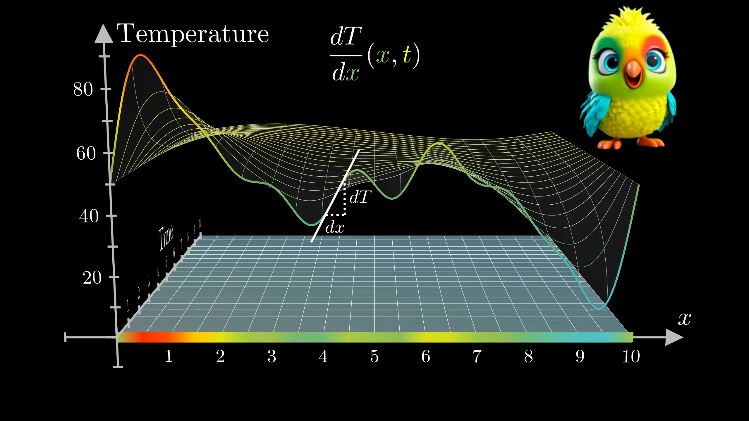
Problem Statement: Heat Conduction in a Rod
A thin rod of length $ L = 1 $ m is initially at a temperature $ u(x,0) = \sin(\pi x) $. The ends of the rod are kept at 0°C for all time $ t > 0 $. The thermal diffusivity is $ \alpha = 1 \, \text{m}^2/\text{s} $.

Find the temperature distribution $ u(x,t) $ for $ t > 0 $.

Mathematical Formulation:
PDE (Heat Equation):
$$
\frac{\partial u}{\partial t} = \alpha \frac{\partial^2 u}{\partial x^2}, \quad 0 < x < 1, \quad t > 0
$$
Initial Condition (IC):
$$
u(x,0) = \sin(\pi x)
$$
Boundary Conditions (BCs):
$$
u(0,t) = 0, \quad u(1,t) = 0
$$

Solution (Separation of Variables)

Step 1: Assume a Separable Solution
Let $ u(x,t) = X(x)T(t) $. Substituting into the PDE:
$$
X(x)T'(t) = \alpha X”(x)T(t)
$$
Divide both sides by $ \alpha X(x)T(t) $:
$$
\frac{T'(t)}{\alpha T(t)} = \frac{X”(x)}{X(x)} = -\lambda
$$
(where $ \lambda $ is a separation constant).

Step 2: Solve the Spatial ODE $ X”(x) + \lambda X(x) = 0 $
Boundary Conditions:
$ X(0) = 0 $ and $ X(1) = 0 $ (from $ u(0,t) = u(1,t) = 0 $).

General Solution:
– If $ \lambda > 0 $, the solution is $ X(x) = A \cos(\sqrt{\lambda}x) + B \sin(\sqrt{\lambda}x) $.
– Applying $ X(0) = 0 $: $ A = 0 $.
– Applying $ X(1) = 0 $: $ B \sin(\sqrt{\lambda}) = 0 $.
– Non-trivial solution requires $ \sin(\sqrt{\lambda}) = 0 $, so $ \sqrt{\lambda} = n\pi $, $ n = 1,2,3,… $
– Thus, eigenvalues: $ \lambda_n = (n\pi)^2 $, and eigenfunctions: $ X_n(x) = \sin(n\pi x) $.

Step 3: Solve the Temporal ODE $ T'(t) + \alpha \lambda_n T(t) = 0 $
For each $ \lambda_n = (n\pi)^2 $:
$$
T_n(t) = C_n e^{-\alpha (n\pi)^2 t}
$$

Step 4: General Solution as a Fourier Series
The general solution is:
$$
u(x,t) = \sum_{n=1}^{\infty} C_n \sin(n\pi x) e^{-(n\pi)^2 t}
$$

Step 5: Apply Initial Condition to Find $ C_n $
At $ t = 0 $:
$$
u(x,0) = \sin(\pi x) = \sum_{n=1}^{\infty} C_n \sin(n\pi x)
$$
This is a Fourier sine series, and since $ \sin(\pi x) $ already matches one term:
– $ C_1 = 1 $
– $ C_n = 0 $ for $ n \geq 2 $

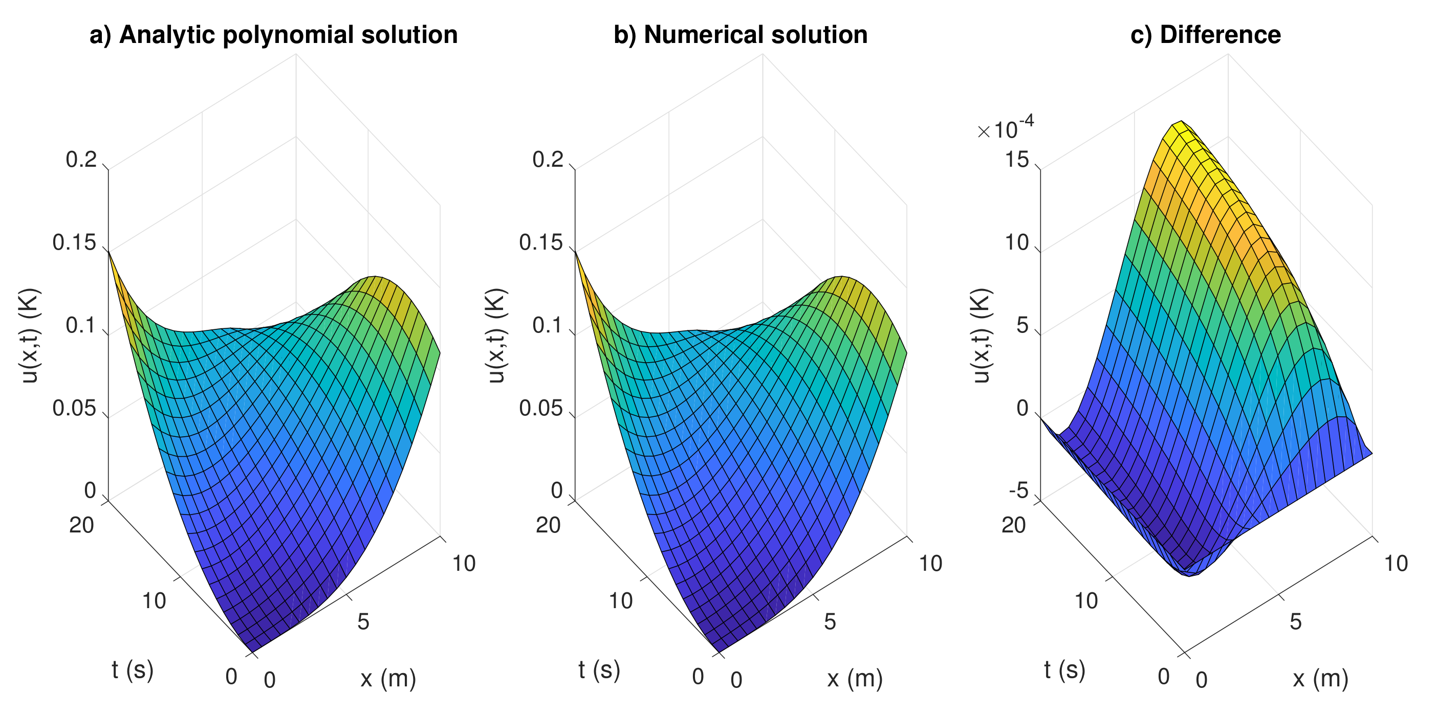
Final Solution:
$$
u(x,t) = \sin(\pi x) e^{-\pi^2 t}
$$

Interpretation:
– The temperature decays exponentially in time while maintaining a sinusoidal shape in space.
– The rate of decay depends on $ \pi^2 $; higher modes (if present) would decay even faster.

Graphical Behavior:
– At $ t = 0 $: $ u(x,0) = \sin(\pi x) $ (peak at $ x = 0.5 $).
– As $ t \to \infty $: $ u(x,t) \to 0 $ (rod cools to 0°C everywhere).

Verification:
– Check PDE:
$ u_t = -\pi^2 e^{-\pi^2 t} \sin(\pi x) $
$ u_{xx} = -\pi^2 e^{-\pi^2 t} \sin(\pi x) $
✓ Satisfies $ u_t = u_{xx} $.

– Check BCs:
$ u(0,t) = 0 $, $ u(1,t) = 0 $ ✓

– Check IC:
$ u(x,0) = \sin(\pi x) $ ✓

Key Takeaways:
The temperature distribution is:
$$
\boxed{u(x,t) = \sin(\pi x) e^{-\pi^2 t}}
$$

– Dirichlet BCs prescribe the value of $ u $ on the boundary.
– Neumann BCs prescribe the derivative (flux) of $ u $ on the boundary.
– Robin BCs mix both (e.g., convective cooling).

Conclusion:

Equation	Type	Discriminant	Application	Historical Figure
Laplace	Elliptic	< 0	Potential fields	Laplace
Heat	Parabolic	= 0	Heat conduction	Fourier
Wave	Hyperbolic	> 0	Sound, vibration	d’Alembert

The classification of PDEs into hyperbolic, parabolic, and elliptic types helps determine solution techniques and physical interpretations. The wave equation governs vibrations, the heat equation models diffusion, and Laplace’s equation describes equilibrium states. These were developed by mathematical giants like d’Alembert, Fourier, and Laplace, shaping modern physics and engineering.