Brief Historical Introduction to Laplace Transform
The Laplace Transform is a cornerstone of mathematical physics and engineering, with deep historical roots dating back to the 18th century. Named after Pierre-Simon Laplace (1749–1827), a French mathematician and astronomer, this transformative tool emerged as part of his work on probability and celestial mechanics.
Origins
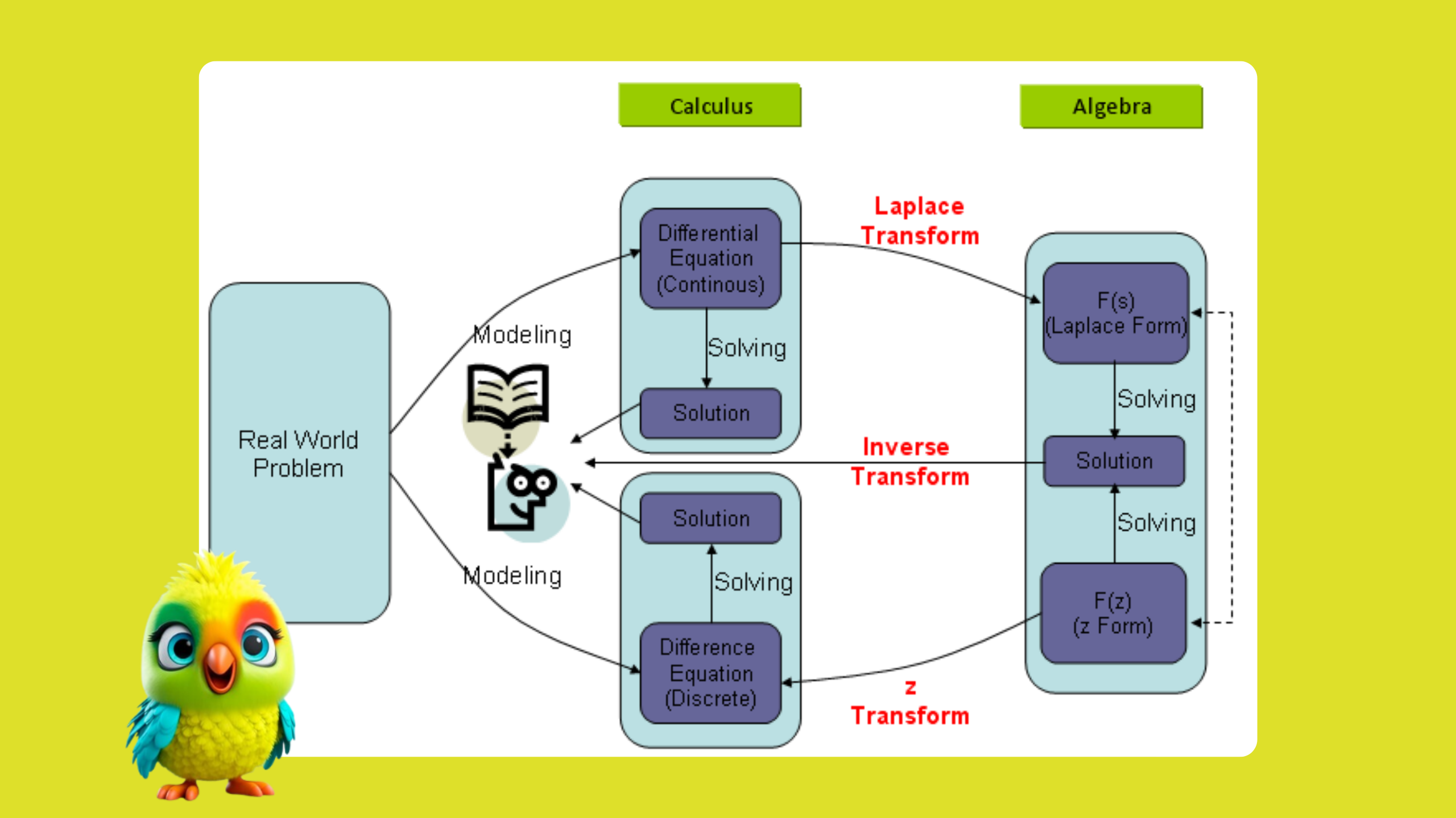
Laplace originally used a form of this integral transformation in his work Théorie analytique des probabilités (1812) to simplify complex differential equations in astronomy and mechanics. His approach aimed to transform differential equations into algebraic equations that were easier to manipulate—a revolutionary concept at the time.
While the concept of transforming functions was not entirely new (Joseph Fourier had earlier developed the Fourier Transform for periodic functions), Laplace’s innovation extended it to a broader class of functions, especially non-periodic and non-stationary signals, making it suitable for exponential growth/decay models.
Evolution Through the Centuries
19th century: Mathematicians like Heaviside in electrical engineering began using operational calculus informally, which later turned out to be formal Laplace transforms.
Early 20th century: The rigorous mathematical foundation was laid down, and the Laplace Transform became standard in solving linear ordinary differential equations (ODEs) and partial differential equations (PDEs).
Modern era: It is now embedded in electrical engineering, control theory, signal processing, quantum mechanics, and increasingly in machine learning (ML) and data science.
Laplace Transform in Machine Learning (ML)
While not as directly prominent as gradient descent or neural networks, Laplace Transforms offer valuable applications in ML—especially in theoretical modeling and signal-based learning systems.
Applications in ML:
- Signal Preprocessing: In ML systems that handle sensor data (e.g., IoT, autonomous vehicles), Laplace transforms help de-noise signals and extract features in the frequency domain.
- System Identification & Control: ML models used in robotics and control systems rely on transfer functions derived via Laplace transforms to understand how systems behave over time.
- Time-Series Forecasting: Laplace Transforms can be used to transform non-stationary time series into domains where patterns are more easily modeled.
- Bayesian Inference (Laplace Approximation): A crucial application: The Laplace approximation helps approximate posterior distributions with Gaussians in probabilistic models, enabling Bayesian neural networks and variational inference.
- Kernel Methods: In support vector machines (SVMs), certain kernels (e.g., Laplacian kernels) are derived from the Laplace transform, affecting decision boundaries and model generalization.
- PDE-Driven Deep Learning: Recent research fuses physics-informed neural networks (PINNs) with Laplace or Fourier transforms to solve PDEs that govern physical processes—blending classical math with AI.
Derivation of the Standard Laplace Equation (∇²u = 0)
The Laplace equation is a second-order partial differential equation (PDE) that arises naturally in physics and engineering. Below is a step-by-step derivation of its standard form.
1. Physical Context
The Laplace equation describes steady-state (time-independent) phenomena where the system is in equilibrium. Examples include:
– Electrostatics: Electric potential \( \phi \) in a charge-free region.
– Fluid Dynamics: Velocity potential \( \psi \) for incompressible, irrotational flow.
– Heat Conduction: Temperature distribution \( T \) in thermal equilibrium.
2. Derivation from Conservation Laws
Case 1: Heat Conduction (Fourier’s Law + Energy Conservation)
1. Fourier’s Law of Heat Conduction:
\[
\mathbf{q} = -k \nabla T
\]
where:
– \( \mathbf{q} \) = heat flux (W/m²),
– \( k \) = thermal conductivity,
– \( \nabla T \) = temperature gradient.
2. Energy Conservation (Divergence of Flux):
\[
\nabla \cdot \mathbf{q} = 0 \quad \text{(Steady state, no heat generation)}
\]
3. Substitute Fourier’s Law:
\[
\nabla \cdot (-k \nabla T) = 0 \implies \nabla^2 T = 0
\]
Case 2: Electrostatics (Gauss’s Law + No Free Charges)
1. Gauss’s Law (Differential Form):
\[
\nabla \cdot \mathbf{E} = \frac{\rho}{\epsilon_0}
\]
where \( \mathbf{E} = -\nabla \phi \).
2. For a charge-free region (\( \rho = 0 \)):
\[
\nabla \cdot (-\nabla \phi) = 0 \implies \nabla^2 \phi = 0
\]
3. Mathematical Formulation
The Laplace operator \( \nabla^2 \) (or Laplacian) in different coordinate systems:
Coordinate System Laplacian \( \nabla^2 u \)
- Cartesian (\( x, y, z \)) | \( \frac{\partial^2 u}{\partial x^2} + \frac{\partial^2 u}{\partial y^2} + \frac{\partial^2 u}{\partial z^2} \)
- Cylindrical (\( r, \theta, z \)) | \( \frac{1}{r} \frac{\partial}{\partial r} \left( r \frac{\partial u}{\partial r} \right) + \frac{1}{r^2} \frac{\partial^2 u}{\partial \theta^2} + \frac{\partial^2 u}{\partial z^2} \)
- Spherical (\( r, \theta, \phi \)) | \( \frac{1}{r^2} \frac{\partial}{\partial r} \left( r^2 \frac{\partial u}{\partial r} \right) + \frac{1}{r^2 \sin \theta} \frac{\partial}{\partial \theta} \left( \sin \theta \frac{\partial u}{\partial \theta} \right) + \frac{1}{r^2 \sin^2 \theta} \frac{\partial^2 u}{\partial \phi^2} \)
4. Intuitive Explanation
The Laplace equation \( \nabla^2 u = 0 \) states that at any point:
– The average value of \( u \) around a small neighborhood equals the value at the center.
– No “sources” or “sinks” are present (unlike the Poisson equation \( \nabla^2 u = f \)).
5. Example Solutions
Cartesian Coordinates (2D):
\[
u(x,y) = e^{ky} \sin(kx)
\]
Verification:
\[
\frac{\partial^2 u}{\partial x^2} = -k^2 u, \quad \frac{\partial^2 u}{\partial y^2} = k^2 u \implies \nabla^2 u = 0
\]
Spherical Symmetry:
\[
u(r) = \frac{C_1}{r} + C_2
\]
Verification:
\[
\nabla^2 u = \frac{1}{r^2} \frac{d}{dr} \left( r^2 \frac{d}{dr} \left( \frac{1}{r} \right) \right) = 0
\]
6. Boundary Conditions
The Laplace equation requires boundary conditions for uniqueness:
1. Dirichlet BC: \( u \) specified on the boundary.
2. Neumann BC: Normal derivative \( \frac{\partial u}{\partial n} \) specified.
3. Robin BC: Mixed condition (e.g., convection).
7. Applications
- Electromagnetics Electric potential in conductors
- Fluid Mechanics Potential flow around obstacles
- Machine Learning Graph Laplacians for semi-supervised learning
- Computer Vision Image inpainting (filling missing pixels)
Key Takeaways
1. The Laplace equation \( \nabla^2 u = 0 \) describes **equilibrium states**.
2. Derived from conservation laws (energy, charge, mass).
3. Solutions depend on coordinate systems and boundary conditions.
4. Extends to Poisson’s equation (\( \nabla^2 u = f \)) when sources exist.
Laplace’s equation is a second-order partial differential equation (PDE) named after Pierre-Simon Laplace. It arises in many areas of physics, including electrostatics, fluid dynamics, and gravitational potential theory.
Derivation from First Principles
1. Gauss’s Law (Electrostatics):
\[
\nabla \cdot \mathbf{E} = \frac{\rho}{\epsilon_0}
\]
For a charge-free region (\( \rho = 0 \)) and \( \mathbf{E} = -\nabla \phi \), we get:
\[
\nabla^2 \phi = 0
\]
2. Heat Conduction (Steady-State):
The heat equation in steady-state (\( \frac{\partial u}{\partial t} = 0 \)) reduces to:
\[
\nabla^2 u = 0
\]
3. Fluid Flow (Irrotational, Incompressible):
If \( \mathbf{v} = \nabla \phi \) and \( \nabla \cdot \mathbf{v} = 0 \), then:
\[
\nabla^2 \phi = 0
\]
General Form (n-Dimensional):
\[
\nabla^2 u = \frac{\partial^2 u}{\partial x_1^2} + \frac{\partial^2 u}{\partial x_2^2} + \dots + \frac{\partial^2 u}{\partial x_n^2} = 0
\]
Part 2: Summary History of Laplace Transforms
Early Origins (1737–1812)
– Leonhard Euler (1737): Introduced integrals of the form \( \int e^{-ax} f(x) \, dx \) to solve differential equations.
– Joseph-Louis Lagrange (1773): Used similar transforms in probability theory.
– Pierre-Simon Laplace (1782): Systematically applied the transform to solve PDEs in celestial mechanics.
Modern Formulation (19th–20th Century)
– Oliver Heaviside (1890s): Popularized operational calculus, a precursor to Laplace transforms.
– Gustav Doetsch (1930s): Rigorously defined the Laplace transform and its inversion.
Key Applications:
1. Electrical Engineering: Solving RLC circuits.
2. Control Theory: Analyzing system stability.
3. Quantum Mechanics: Time-independent Schrödinger equation.
Part 3: Laplace Transforms with Examples
1. Standard Laplace Transform
\[
\mathcal{L}\{f(t)\} = F(s) = \int_0^\infty e^{-st} f(t) \, dt
\]
Example 1 (Simple):
\[
f(t) = e^{at} \implies F(s) = \frac{1}{s-a}, \quad \text{Re}(s) > a
\]
Example 2 (Difficult):
\[
f(t) = t \sin(at) \implies F(s) = \frac{2as}{(s^2 + a^2)^2}
\]
(Requires integration by parts and frequency differentiation.)
2. Inverse Laplace Transform
\[
\mathcal{L}^{-1}\{F(s)\} = f(t) = \frac{1}{2\pi i} \lim_{T \to \infty} \int_{\gamma – iT}^{\gamma + iT} e^{st} F(s) \, ds
\]
Example 1 (Simple):
\[
F(s) = \frac{1}{s^2} \implies f(t) = t
\]
Example 2 (Complex):
\[
F(s) = \frac{e^{-s}}{s^2 + \pi^2} \implies f(t) = \frac{1}{\pi} \sin(\pi (t-1)) \cdot u(t-1)
\]
(Requires contour integration and Heaviside shift.)
3. Two-Sided (Bilateral) Laplace Transform
\[
\mathcal{B}\{f(t)\} = \int_{-\infty}^\infty e^{-st} f(t) \, dt
\]
Example 1 (Simple):
\[
f(t) = e^{-a|t|} \implies F(s) = \frac{2a}{a^2 – s^2}, \quad -a < \text{Re}(s) < a
\]
Example 2 (Difficult):
\[
f(t) = \text{sinc}(t) = \frac{\sin t}{t} \implies F(s) = \pi \cdot \text{rect}(s/2)
\]
(Uses Fourier duality and requires complex analysis.)
4. Fractional Laplace Transform
\[
\mathcal{L}_\alpha\{f(t)\} = \int_0^\infty e^{-s t^\alpha} f(t) \, dt
\]
Example 1 (Simple):
\[
f(t) = t^{\beta} \implies F(s) = \frac{\Gamma(\beta + 1)}{s^{\beta + 1}}
\]
Example 2 (Complex):
\[
f(t) = E_\alpha(-t^\alpha) \quad (\text{Mittag-Leffler function})
\]
(Solution involves Fox H-functions.)
Key Takeaways:
1. Laplace’s Equation: Governs steady-state phenomena.
2. Laplace Transforms:
– Standard: Solves ODEs/PDEs via algebraic manipulation.
– Inverse: Requires contour integration.
– Bilateral: Handles non-causal signals.
– Fractional: Extends to anomalous diffusion.
3. Historical Impact: From celestial mechanics to quantum fields.
Derivation of Laplace Transforms for Common Functions Continuation
We derive the Laplace transforms for \( x \), \( c \), \( \sin x \), and \( \cos x \) using the definition:
\[
\mathcal{L}\{f(x)\} = F(s) = \int_0^\infty e^{-sx} f(x) \, dx
\]
1. Laplace Transform of \( f(x) = c \) (Constant Function)
Derivation:
\[
\mathcal{L}\{c\} = \int_0^\infty e^{-sx} c \, dx = c \int_0^\infty e^{-sx} \, dx = c \left[ \frac{-e^{-sx}}{s} \right]_0^\infty = \frac{c}{s}
\]
Examples:
– Simple:
\[
\mathcal{L}\{5\} = \frac{5}{s}
\]
– Complex:
\[
\mathcal{L}\{c \cdot u(x-a)\} = \frac{c e^{-as}}{s} \quad \text{(Heaviside shift)}
\]
2. Laplace Transform of \( f(x) = x \) (Linear Function)
Derivation:
\[
\mathcal{L}\{x\} = \int_0^\infty e^{-sx} x \, dx
\]
Using integration by parts (\( u = x \), \( dv = e^{-sx} \, dx \)):
\[
= \left[ \frac{-x e^{-sx}}{s} \right]_0^\infty + \frac{1}{s} \int_0^\infty e^{-sx} \, dx = \frac{1}{s^2}
\]
Examples:
– Simple:
\[
\mathcal{L}\{3x\} = \frac{3}{s^2}
\]
– Complex:
\[
\mathcal{L}\{x e^{ax}\} = \frac{1}{(s-a)^2} \quad \text{(Frequency shift)}
\]
3. Laplace Transform of \( f(x) = \sin x \)
Derivation:
\[
\mathcal{L}\{\sin x\} = \int_0^\infty e^{-sx} \sin x \, dx
\]
Using integration by parts twice (or complex exponentials):
\[
= \left. \frac{-e^{-sx} (s \sin x + \cos x)}{s^2 + 1} \right|_0^\infty = \frac{1}{s^2 + 1}
\]
Examples:
– Simple:
\[
\mathcal{L}\{\sin 2x\} = \frac{2}{s^2 + 4}
\]
– Complex:
\[
\mathcal{L}\{e^{-x} \sin x\} = \frac{1}{(s+1)^2 + 1} \quad \text{(Damped sine)}
\]
4. Laplace Transform of \( f(x) = \cos x \)
Derivation:
\[
\mathcal{L}\{\cos x\} = \int_0^\infty e^{-sx} \cos x \, dx
\]
Again, integration by parts:
\[
= \left. \frac{e^{-sx} (s \cos x – \sin x)}{s^2 + 1} \right|_0^\infty = \frac{s}{s^2 + 1}
\]
Examples:
– Simple:
\[
\mathcal{L}\{\cos 3x\} = \frac{s}{s^2 + 9}
\]
– Complex:
\[
\mathcal{L}\{x \cos x\} = \frac{s^2 – 1}{(s^2 + 1)^2} \quad \text{(Multiplication by \( x \))}
\]
5. Basic Transform: \( f(t) = t^2 \)
Derivation:
Using the definition:
\[
\mathcal{L}\{t^2\} = \int_0^\infty e^{-st} t^2 \, dt
\]
Integration by parts (\( u = t^2 \), \( dv = e^{-st} dt \)):
\[
= \left[ \frac{-t^2 e^{-st}}{s} \right]_0^\infty + \frac{2}{s} \int_0^\infty t e^{-st} \, dt
\]
The first term vanishes at \( t \to \infty \), and the second integral is \( \mathcal{L}\{t\} = \frac{1}{s^2} \):
\[
= \frac{2}{s} \cdot \frac{1}{s^2} = \frac{2}{s^3}
\]
Difficult Example: \( f(t) = t^2 e^{-3t} \)
Using frequency shift (\( \mathcal{L}\{e^{at} f(t)\} = F(s-a) \)):
\[
\mathcal{L}\{t^2 e^{-3t}\} = \left. \frac{2}{s^3} \right|_{s \to s+3} = \frac{2}{(s+3)^3}
\]
Complex Example: \( f(t) = t^2 \sin(at) \)
Using \( \mathcal{L}\{\sin(at)\} = \frac{a}{s^2 + a^2} \) and the property \( \mathcal{L}\{t^n f(t)\} = (-1)^n \frac{d^n}{ds^n} F(s) \):
\[
\mathcal{L}\{t^2 \sin(at)\} = \frac{d^2}{ds^2} \left( \frac{a}{s^2 + a^2} \right) = \frac{2as(s^2 – 3a^2)}{(s^2 + a^2)^3}
\]
6. Exponential Multiplication: \( f(t) = e^{at} \)
Derivation:
\[
\mathcal{L}\{e^{at}\} = \int_0^\infty e^{-st} e^{at} \, dt = \int_0^\infty e^{-(s-a)t} \, dt = \frac{1}{s-a}, \quad s > a
\]
Difficult Example: \( f(t) = t e^{4t} \)
Using \( \mathcal{L}\{t f(t)\} = -\frac{d}{ds} F(s) \):
\[
\mathcal{L}\{t e^{4t}\} = -\frac{d}{ds} \left( \frac{1}{s-4} \right) = \frac{1}{(s-4)^2}
\]
Complex Example: \( f(t) = t \cos(bt) e^{-at} \)
First, find \( \mathcal{L}\{\cos(bt)\} = \frac{s}{s^2 + b^2} \). Apply frequency shift (\( s \to s+a \)):
\[
\mathcal{L}\{\cos(bt) e^{-at}\} = \frac{s+a}{(s+a)^2 + b^2}
\]
Then multiply by \( t \):
\[
\mathcal{L}\{t \cos(bt) e^{-at}\} = -\frac{d}{ds} \left( \frac{s+a}{(s+a)^2 + b^2} \right) = \frac{(s+a)^2 – b^2}{[(s+a)^2 + b^2]^2}
\]
7. Unit Step Function: \( f(t) = u(t-a) \)
Derivation:
\[
\mathcal{L}\{u(t-a)\} = \int_a^\infty e^{-st} \, dt = \frac{e^{-as}}{s}
\]
Difficult Example: \( f(t) = (t-2)^2 u(t-2) \)
Using time shift (\( \mathcal{L}\{f(t-a) u(t-a)\} = e^{-as} F(s) \)):
\[
\mathcal{L}\{(t-2)^2 u(t-2)\} = e^{-2s} \mathcal{L}\{t^2\} = \frac{2 e^{-2s}}{s^3}
\]
Complex Example: \( f(t) = e^{3(t-1)} \sin(2(t-1)) u(t-1) \)
First, find \( \mathcal{L}\{\sin(2t)\} = \frac{2}{s^2 + 4} \). Apply time shift (\( t \to t-1 \)) and frequency shift (\( s \to s-3 \)):
\[
\mathcal{L}\{e^{3(t-1)} \sin(2(t-1)) u(t-1)\} = e^{-s} \left. \frac{2}{s^2 + 4} \right|_{s \to s-3} = \frac{2 e^{-s}}{(s-3)^2 + 4}
\]
Part 2: Key Observations
1. Linearity:
\[
\mathcal{L}\{a f(t) + b g(t)\} = a F(s) + b G(s)
\]
2. Frequency Shift:
\[
\mathcal{L}\{e^{at} f(t)\} = F(s-a)
\]
3. Time Shift:
\[
\mathcal{L}\{f(t-a) u(t-a)\} = e^{-as} F(s)
\]
4. Multiplication by \( t^n \):
\[
\mathcal{L}\{t^n f(t)\} = (-1)^n \frac{d^n}{ds^n} F(s)
\]
Final Notes
– For \( t^n \): Repeated differentiation of \( \frac{1}{s} \).
– For oscillatory functions: Combine with exponential shifts for damped cases.
– For piecewise functions: Use unit step (\( u(t-a) \)) and time shifts.
Key Observations:
1. Linearity:
\[
\mathcal{L}\{a f(x) + b g(x)\} = a F(s) + b G(s)
\]
2. Frequency Shift:
\[
\mathcal{L}\{e^{ax} f(x)\} = F(s-a)
\]
3. Time Shift:
\[
\mathcal{L}\{f(x-a) u(x-a)\} = e^{-as} F(s)
\]
Final Notes
– For \( x^n \): Repeated integration by parts gives \( \mathcal{L}\{x^n\} = \frac{n!}{s^{n+1}} \).
– For hyperbolic functions:
\[
\mathcal{L}\{\sinh x\} = \frac{1}{s^2 – 1}, \quad \mathcal{L}\{\cosh x\} = \frac{s}{s^2 – 1}
\]


