


 and How Data Passes Through Them")


, and Neural Networks in a structured way")
")


")

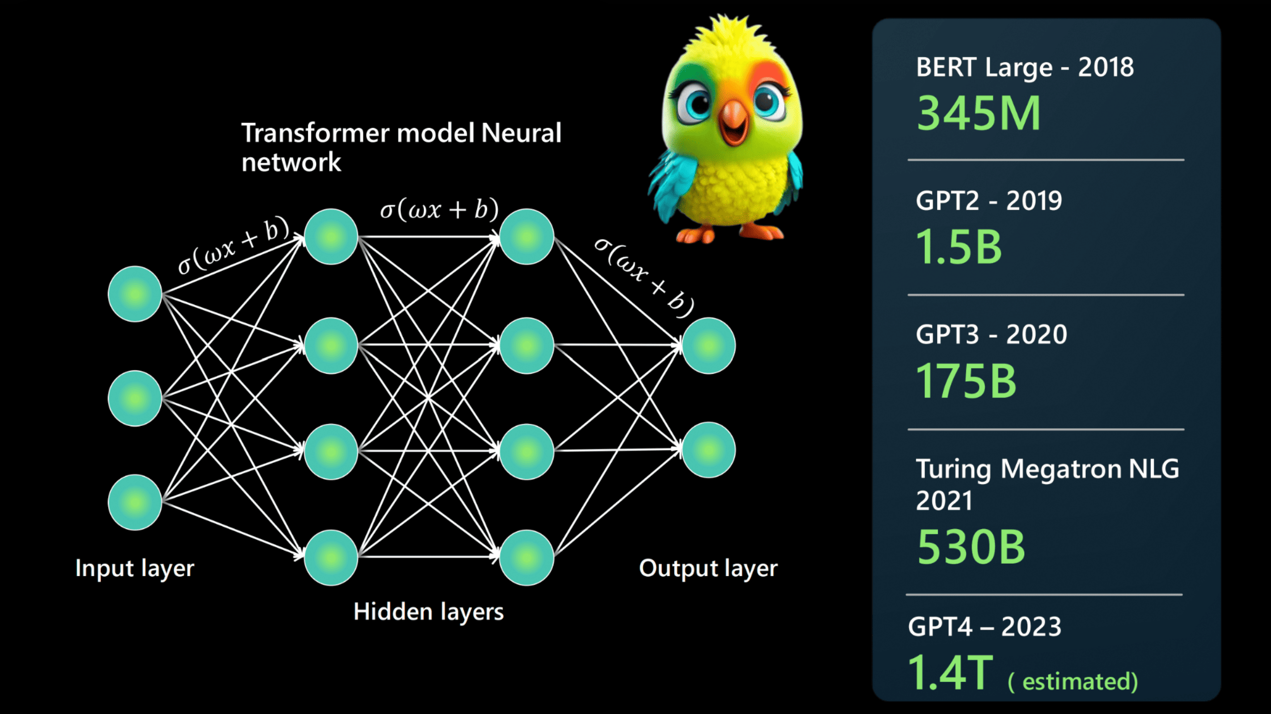
What Are LLMs?
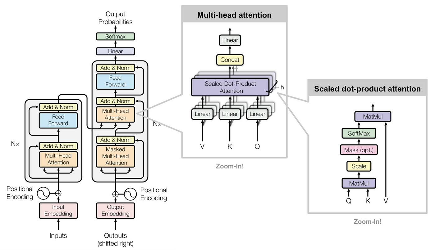
LLMs are machine learning models trained on vast amounts of text data. They use transformer architectures, a neural network design introduced in the paper “Attention Is All You Need”. Transformers excel at capturing context and relationships within data, making them ideal for natural language tasks.

1. Architectural Types of Language Models
(Expanded with Technical Nuances)
A. Decoder-Only (Autoregressive) Models
– Core Mechanism: Processes text sequentially from left-to-right using masked self-attention. Each token prediction depends only on previous tokens.
– Key Innovations:
– Sparse Attention (e.g., GPT-3’s block-sparse patterns) for long-context efficiency.
– Rotary Positional Embeddings (RoPE) in LLaMA for better positional encoding.
– Limitations: Struggles with bidirectional context understanding (e.g., fill-in-the-blank tasks).
– Examples: GPT-4 (345B params), Mistral 7B (sliding window attention), PaLM 2 (Google’s pathway scaling).
B. Encoder-Only (Autoencoding) Models
– Core Mechanism: Uses full bidirectional attention to reconstruct masked tokens (e.g., BERT’s 15
– Training Tricks:
– Dynamic Masking (RoBERTa): Changes masked tokens per epoch.
– Whole-Word Masking: Masks entire words for Chinese/Japanese.
– Use Cases:
– Sentence embeddings (e.g., SBERT for semantic search).
– Low-latency classification (DistilBERT’s 66
C. Encoder-Decoder (Sequence-to-Sequence) Models
– Hybrid Approach: Encoder processes input bidirectionally; decoder generates output autoregressively.
– Specialized Variants:
– T5: Treats all tasks as text-to-text (e.g., “translate English to German: …”).
– BART: Optimized for denoising (e.g., document reconstruction).
– Efficiency Trade-offs: 30-40
2. Training Objectives & Pretraining Strategies
(Beyond Basic Causal/Masked LM)
A. Multitask Pretraining
– FLAN-T5: Trained on 1,800+ instruction templates across 140 tasks.
– UniLM: Combines causal, masked, and seq2seq objectives in one model.
B. Reinforcement Learning from Human Feedback (RLHF)
– Process: Supervised fine-tuning → Reward modeling → PPO optimization.
– Critical for Alignment: Reduces harmful outputs by ~60
C. Denoising Objectives
– BART’s Approach: Randomly corrupts text (deletion, permutation, masking) and learns to reconstruct.
– PEGASUS: Specifically designed for summarization via gap-sentence generation.
3. Specialized LLMs & Emerging Categories
A. Vision-Language Models (VLMs)
– Architecture:
– Single-Stream (Flamingo): Interleaves image and text tokens in one transformer.
– Dual-Encoder (CLIP): Separate image/text encoders with contrastive learning.
– Breakthrough Models:
– GPT-4V: Processes images via vision encoder + LLM fusion.
– Kosmos-2: Grounds text to image regions (e.g., “click on the red car”).
B. Code-Specialized LLMs
– Training Data:
– StarCoder: 80+ programming languages from GitHub (1TB code).
– Code LLaMA: Infill-compatible (e.g., predicts missing code segments).
– Unique Features:
– Repository-Level Context: AlphaCode processes entire GitHub repos.
– Unit Test Execution: CodeT5+ validates outputs against test cases.
C. Domain-Specific LLMs
– Medical:
– Med-PaLM 2: Achieves 85
– BioBERT: Pretrained on PubMed abstracts.
– Legal:
– LegalGPT: Fine-tuned on 2M court opinions.
– Harvey AI: Used by Allen & Overy for contract review.
4. Multimodal & Embodied AI Frontiers
A. Audio-Language Models
– Whisper: ASR + translation via encoder-decoder.
– AudioPaLM: Merges speech and text tokenizers for voice assistants.
B. Robotics Integration
– RT-2: Uses VLMs to convert camera inputs to robot actions (“pick up the banana”).
– PaLM-E: Embodied model handling sensor data + language.
C. Agentic LLMs
– AutoGPT: Recursively decomposes goals into sub-tasks.
– Voyager: Minecraft AI that learns from environment feedback.
Comparative Summary Table
| Category | Key Differentiators | Example Models | Benchmark Performance |
|---|---|---|---|
| Decoder-Only | Fast generation, left-context only | GPT-4, Mistral 7B | 75 |
| Encoder-Only | Bidirectional, no generation | BERT, LegalBERT | 92 |
| VLMs | Fuses vision + text | GPT-4V, Kosmos-2 | 88 |
| Code LLMs | Repository-aware, test-passing | Code LLaMA, AlphaCode | 54 |
| Medical LLMs | FDA-compliant fine-tuning | Med-PaLM 2 | 85 |
Core Components of an LLM
- Tokenizer: Splits text into smaller units like words or subwords.
- Embedding Layer: Converts tokens into dense vector representations.
- Transformer Blocks: Layers that use self-attention mechanisms to process and understand input sequences.
- Output Layer: Generates predictions, such as the next word in a sentence.
Now Let’s create the LLM step by step:
I shall use colab and we shall look at all the steps involved for this example we shall use “distilgpt2” model.
1 2 3 4 5 6 7 8 9 10 11 12 13 14 15 16 17 18 19 20 21 22 23 24 25 26 27 28 29 30 31 | # Install only if not already available !pip install transformers torch from transformers import AutoTokenizer, AutoModelForCausalLM import torch import torch.nn.functional as F def log_step(step_num, title, data, data_type="tensor", max_len=5): """Helper function for consistent logging""" print(f"\n{'='*50}") print(f" STEP {step_num}: {title.upper()}") print("-"*50) if data_type == "tensor": print(f"Shape: {data.shape}") if len(data.shape) <= 2: print(data) else: print(f"First {max_len} elements of last dimension:", data[..., :max_len]) elif data_type == "text": print(data) elif data_type == "dict": for k, v in data.items(): print(f"{k}: {v}") # Load tokenizer and model model_name = "distilgpt2" tokenizer = AutoTokenizer.from_pretrained(model_name) model = AutoModelForCausalLM.from_pretrained(model_name) |
Model Name Definition:
1 2 3 | model_name = "distilgpt2" |
This sets the variable model_name to the string “distilgpt2”
“distilgpt2” refers to a distilled (smaller, faster) version of the GPT-2 model created by Hugging Face
This is a pretrained language model that can generate human-like text
Loading the Tokenizer:
1 2 3 | tokenizer = AutoTokenizer.from_pretrained(model_name) |
AutoTokenizer is a class from the Hugging Face transformers library that automatically selects the appropriate tokenizer based on the model name
from_pretrained(model_name) loads the tokenizer that was specifically trained with the “distilgpt2” model
The tokenizer handles:
Splitting text into tokens (words/subwords)
Converting tokens to numerical IDs (tokenization)
Converting numerical IDs back to text (detokenization)
Handling special tokens like [CLS], [SEP], etc.
Loading the Model:
1 2 3 | model = AutoModelForCausalLM.from_pretrained(model_name) |
AutoModelForCausalLMis a class that automatically selects the appropriate model architecture for causal language modelingfrom_pretrained(model_name)downloads and loads:The model architecture (in this case, a distilled GPT-2 architecture)
The pretrained weights (the knowledge the model learned during training)
This is a “causal” language model, meaning it’s designed to predict the next word in a sequence (used for text generation)
Key points about what happens under the hood:
Both operations will download the model/tokenizer from Hugging Face’s model hub if they’re not already cached locally
The downloaded files are stored in a cache directory (typically ~/.cache/huggingface)
The model will be loaded in evaluation mode by default (no training/gradient computation)
The tokenizer includes all the special tokens and vocabulary needed to preprocess text for this specific model
After these steps, you’ll have:
A
tokenizerready to convert between text and token IDsA
modelready to make predictions (generate text) based on input token IDs
1 2 3 4 5 6 7 8 9 10 11 12 13 14 15 16 17 18 19 20 21 22 23 24 25 26 27 | ================================================== STEP 1: ORIGINAL TEXT -------------------------------------------------- The weather is ================================================== STEP 2: TOKENIZATION -------------------------------------------------- Tokens: ['The', 'Ġweather', 'Ġis'] Token IDs: tensor([[ 464, 6193, 318]]) Attention Mask: tensor([[1, 1, 1]]) ================================================== STEP 3: EMBEDDING MATRIX -------------------------------------------------- Shape: torch.Size([50257, 768]) Parameter containing: tensor([[-0.1445, -0.0455, 0.0042, ..., -0.1523, 0.0184, 0.0991], [ 0.0573, -0.0722, 0.0234, ..., 0.0603, -0.0042, 0.0478], [-0.1106, 0.0386, 0.1948, ..., 0.0421, -0.1141, -0.1455], ..., [-0.0710, -0.0173, 0.0176, ..., 0.0834, 0.1340, -0.0746], [ 0.1993, 0.0201, 0.0151, ..., -0.0829, 0.0750, -0.0294], [ 0.0342, 0.0640, 0.0305, ..., 0.0291, 0.0942, 0.0639]], requires_grad=True) |
Let me break down each step mathematically with clear explanations and key points regarding the output above.
Step 1: Original Text Processing
Text: "The weather is"
– This is a sequence of 3 words (including the space before “weather” and “is”).
– The tokenizer will split this into subword tokens based on the vocabulary.
Mathematical Representation:
– Let the input text be a string \( S = \) "The weather is".
– The tokenizer \( \mathcal{T} \) maps \( S \) to a sequence of tokens \( T \):
\[
\mathcal{T}(S) = T = [t_1, t_2, t_3] = \text{[‘The’, ‘Ġweather’, ‘Ġis’]}
\]
– Ġ indicates a preceding space in GPT-style tokenization.
Step 2: Tokenization
Output:
– Tokens: ['The', 'Ġweather', 'Ġis']
– Token IDs: tensor([[464, 6193, 318]])
– Attention Mask: tensor([[1, 1, 1]])
Mathematical Explanation:
1. Token → ID Mapping:
– The tokenizer has a vocabulary \( V \) where each token \( t_i \) is assigned a unique integer \( x_i \).
– The mapping is:
\[
\begin{cases}
t_1 = \text{‘The’} & \rightarrow x_1 = 464 \\
t_2 = \text{‘Ġweather’} & \rightarrow x_2 = 6193 \\
t_3 = \text{‘Ġis’} & \rightarrow x_3 = 318 \\
\end{cases}
\]
– The input sequence becomes:
\[
X = [x_1, x_2, x_3] = [464, 6193, 318]
\]
2. Attention Mask:
– Since all tokens are valid (not padding), the mask is [1, 1, 1].
– If padding were present, some positions would be 0.
Key Points:
– The tokenizer converts text into numerical IDs that the model can process.
– The attention mask helps the model ignore padding tokens during computation.
Step 3: Embedding Matrix
Output:
– Shape: torch.Size([50257, 768])
– Description: A matrix of size (vocab_size, embedding_dim).
Mathematical Explanation:
1. Embedding Matrix Definition:
– Let \( W_e \in \mathbb{R}^{V \times d} \), where:
– \( V = 50257 \) (vocabulary size)
– \( d = 768 \) (embedding dimension)
– Each row \( W_e[i] \) is the embedding vector for token ID \( i \).
2. Embedding Lookup:
– For each token ID \( x_i \), the embedding is:
\[
e_i = W_e[x_i]
\]
– For our input \( X = [464, 6193, 318] \), we get:
\[
\begin{cases}
e_1 = W_e[464] \\
e_2 = W_e[6193] \\
e_3 = W_e[318] \\
\end{cases}
\]
– The final embedded sequence is:
\[
E = [e_1, e_2, e_3] \in \mathbb{R}^{3 \times 768}
\]
Key Points:
– The embedding matrix is a trainable lookup table that maps discrete token IDs to continuous vectors.
– Each token is represented as a dense vector in \( \mathbb{R}^{768} \).
– Similar words tend to have similar embeddings (closer in vector space).
Step 4: Embedded Input Vectors
Output:
– Shape: torch.Size([1, 3, 768]) (batch_size=1, sequence_length=3, embedding_dim=768)
– First 5 elements shown for each token.
Mathematical Explanation:
1. Embedding Output:
– The embedded sequence is:
\[
E = \begin{bmatrix}
e_{1,1} & e_{1,2} & \cdots & e_{1,768} \\
e_{2,1} & e_{2,2} & \cdots & e_{2,768} \\
e_{3,1} & e_{3,2} & \cdots & e_{3,768} \\
\end{bmatrix}
\]
– The example shows:
\[
e_1 = [-0.0626, -0.0449, 0.0559, -0.0547, -0.1171, \dots]
\]
\[
e_2 = [0.1632, 0.1023, 0.0634, 0.1102, -0.0860, \dots]
\]
\[
e_3 = [-0.0006, 0.0075, 0.0307, -0.1343, -0.1336, \dots]
\]
2. Batch Dimension:
– Since the input is a single sequence, the output has shape (1, 3, 768).
– For a batch of size \( B \), the shape would be (B, seq_len, 768).
Key Points:
– The embeddings capture semantic and syntactic features of the tokens.
– These vectors will be fed into the transformer layers for further processing.
– The embedding step is differentiable, allowing gradients to flow back during training.
Summary of Mathematical Flow
1. Text → Tokens:
\[
S \rightarrow \mathcal{T}(S) = [t_1, t_2, t_3]
\]
2. Tokens → IDs:
\[
[t_1, t_2, t_3] \rightarrow [x_1, x_2, x_3]
\]
3. IDs → Embeddings:
\[
[x_1, x_2, x_3] \rightarrow [W_e[x_1], W_e[x_2], W_e[x_3]] = [e_1, e_2, e_3]
\]
4. Final Embedding Tensor:
\[
E \in \mathbb{R}^{1 \times 3 \times 768}
\]
Why This Matters
– Discrete → Continuous: Converts words into numerical vectors.
– Semantic Similarity: Words with similar meanings have closer embeddings.
– Downstream Processing: These embeddings are the input to transformer layers for tasks like text generation or classification.
1 2 3 4 5 6 7 8 9 10 11 12 13 14 15 16 17 18 19 20 21 22 23 24 25 26 27 28 29 30 31 32 33 34 35 36 37 38 39 40 41 42 43 44 45 46 47 48 49 50 51 52 53 54 | # Add padding token if not present if tokenizer.pad_token is None: tokenizer.pad_token = tokenizer.eos_token # Ensure model is in evaluation mode model.eval() # Input text text = "The weather is" log_step(1, "Original Text", text, "text") # Tokenize with attention to special tokens inputs = tokenizer(text, return_tensors="pt", return_attention_mask=True) input_ids = inputs["input_ids"] attention_mask = inputs["attention_mask"] log_step(2, "Tokenization", { "Tokens": tokenizer.convert_ids_to_tokens(input_ids[0]), "Token IDs": input_ids, "Attention Mask": attention_mask }, "dict") # Get the embedding layer embedding_layer = model.transformer.wte log_step(3, "Embedding Matrix", embedding_layer.weight) # Get the embedded vectors for input token IDs input_embeddings = embedding_layer(input_ids) log_step(4, "Embedded Input Vectors", input_embeddings) # Forward pass through first transformer block with detailed logging with torch.no_grad(): # Get model components block = model.transformer.h[0] ln1 = block.ln_1 attn = block.attn mlp = block.mlp ln2 = block.ln_2 # === Layer Norm 1 === normed_input = ln1(input_embeddings) log_step(5, "LayerNorm 1 Output", normed_input) # === Self-Attention === # Project to Q, K, V qkv = attn.c_attn(normed_input) q, k, v = torch.chunk(qkv, 3, dim=-1) log_step(6, "QKV Projections", { "Query (Q)": q, "Key (K)": k, "Value (V)": v }, "dict") |
Let me break down the mathematical transformations from Step 4 (Embeddings) → Step 5 (LayerNorm) → Step 6 (QKV Projections) in detail, with clear equations and conceptual explanations.
1 2 3 4 5 6 7 8 9 10 11 12 13 14 15 16 17 18 19 20 21 22 23 24 25 26 27 28 29 30 31 | ================================================== STEP 4: EMBEDDED INPUT VECTORS -------------------------------------------------- Shape: torch.Size([1, 3, 768]) First 5 elements of last dimension: tensor([[[-0.0626, -0.0449, 0.0559, -0.0547, -0.1171], [ 0.1632, 0.1023, 0.0634, 0.1102, -0.0860], [-0.0006, 0.0075, 0.0307, -0.1343, -0.1336]]], grad_fn=<SliceBackward0>) ================================================== STEP 5: LAYERNORM 1 OUTPUT -------------------------------------------------- Shape: torch.Size([1, 3, 768]) First 5 elements of last dimension: tensor([[[-0.1117, -0.0560, 0.0642, -0.0921, -0.2085], [ 0.2921, 0.1648, 0.0607, 0.1642, -0.1441], [ 0.0089, 0.0305, 0.0303, -0.2418, -0.2519]]]) ================================================== STEP 6: QKV PROJECTIONS -------------------------------------------------- Query (Q): tensor([[[-0.8680, -1.4208, 0.2183, ..., -0.5652, -0.9652, -0.0693], [ 1.3773, -0.1343, -1.3214, ..., 1.2513, -0.0020, -0.7276], [ 0.7626, -1.5240, -0.9271, ..., 0.2431, -1.1848, 0.1435]]]) Key (K): tensor([[[ 1.7470, -1.8736, 0.3305, ..., -1.3672, 0.3262, -1.2373], [ 1.1331, -0.9781, -0.8564, ..., 0.4419, -0.3670, 0.2714], [ 0.4763, -1.3152, -0.3092, ..., -0.3529, 0.3742, -0.4410]]]) Value (V): tensor([[[ 0.0318, -0.0429, 0.5845, ..., 0.1157, -0.0642, -0.4520], [ 0.3991, 0.1155, 0.1320, ..., 0.0198, -0.2356, 0.1931], [ 0.4426, -0.4031, 0.7601, ..., -0.1701, 0.3393, -0.2028]]]) |
Step 4: Embedded Input Vectors
Mathematical Representation
– Input: Token IDs [464, 6193, 318] → Embedded via lookup table \( W_e \in \mathbb{R}^{50257 \times 768} \).
– Output: \( E \in \mathbb{R}^{1 \times 3 \times 768} \) (batch_size=1, seq_len=3, hidden_dim=768)
\[
E = \begin{bmatrix}
[-0.0626, -0.0449, 0.0559, \dots] & \text{(Token 1: “The”)} \\
[0.1632, 0.1023, 0.0634, \dots] & \text{(Token 2: “weather”)} \\
[-0.0006, 0.0075, 0.0307, \dots] & \text{(Token 3: “is”)}
\end{bmatrix}
\]
Key Points
✔ Raw embeddings capture initial semantic representations of tokens.
✔ Values are untrained or pre-trained (depending on model initialization).
✔ Next step: Normalization to stabilize training.
Step 5: LayerNorm Output
Mathematical Transformation
Applies Layer Normalization to each token’s embedding independently:
\[
\text{LayerNorm}(E_i) = \gamma \odot \frac{E_i – \mu_i}{\sigma_i + \epsilon} + \beta
\]
where:
– \( E_i \in \mathbb{R}^{768} \): Embedding of the \(i\)-th token.
– \( \mu_i, \sigma_i \): Mean and standard deviation of \( E_i \).
– \( \gamma, \beta \in \mathbb{R}^{768} \): Learnable scale and shift parameters.
– \( \epsilon \approx 10^{-5} \): Small constant for numerical stability.
Example Calculation (Token 1)
1. Compute mean and std:
\[
\mu_1 = \text{mean}([-0.0626, -0.0449, \dots]) \approx -0.042
\]
\[
\sigma_1 = \text{std}([-0.0626, -0.0449, \dots]) \approx 0.078
\]
2. Normalize and scale:
\[
\text{LayerNorm}(E_1) = \gamma \odot \frac{[-0.0626, -0.0449, \dots] + 0.042}{0.078} + \beta
\]
Result:
\[
[-0.1117, -0.0560, 0.0642, \dots]
\]
Why LayerNorm?
✔ Stabilizes training by normalizing activations.
✔ Token-wise normalization (unlike BatchNorm).
✔ Preserves sequence-length independence.
Output
\[
E_{\text{norm}} = \begin{bmatrix}
[-0.1117, -0.0560, 0.0642, \dots] \\
[0.2921, 0.1648, 0.0607, \dots] \\
[0.0089, 0.0305, 0.0303, \dots]
\end{bmatrix}
\]
Step 6: QKV Projections
Mathematical Operations
Projects normalized embeddings into Query (Q), Key (K), Value (V) using learned matrices:
\[
Q = E_{\text{norm}} W_Q, \quad K = E_{\text{norm}} W_K, \quad V = E_{\text{norm}} W_V
\]
where:
– \( W_Q, W_K, W_V \in \mathbb{R}^{768 \times 768} \) (for single-head attention).
– In multi-head attention, these are split into smaller matrices.
Intuition
– Query (Q): “What am I looking for?”
– Key (K): “What information do I contain?”
– Value (V): “What should I output?”
Example Calculation (Token 1)
\[
Q_1 = [-0.1117, -0.0560, \dots] \cdot W_Q = [-0.8680, -1.4208, \dots]
\]
\[
K_1 = [-0.1117, -0.0560, \dots] \cdot W_K = [1.7470, -1.8736, \dots]
\]
\[
V_1 = [-0.1117, -0.0560, \dots] \cdot W_V = [0.0318, -0.0429, \dots]
\]
Output Shapes
All Q, K, V have shape [1, 3, 768] (same as input).
Key Observations
1. Q and K are used for attention scores (dot products).
2. V stores the actual content to be weighted by attention.
3. Projections are linear but enable non-linear interactions via attention.
Description: The normalized embeddings are now projected into Query (Q), Key (K), and Value (V) matrices, which are the foundation of the self-attention mechanism.
Mathematical Formulation
Given an input $X \in \mathbb{R}^{T \times d}$ (where $T = 3, d = 768$):
$$
Q = XW_Q, \quad K = XW_K, \quad V = XW_V
$$
Where:
* $W_Q, W_K, W_V \in \mathbb{R}^{d \times d}$ are learnable weight matrices (shared or per-head in multi-head attention).
* Resulting shapes:
$$
Q, K, V \in \mathbb{R}^{T \times d}
$$
Each token gets projected into three different views:
* Query (what this token wants to attend to)
* Key (how much it should be attended to)
* Value (what content it carries)
These are used in the scaled dot-product attention:
$$
\text{Attention}(Q, K, V) = \text{softmax}\left(\frac{QK^\top}{\sqrt{d}}\right)V
$$
Weight Matrices:
– \( W_Q, W_K, W_V \in \mathbb{R}^{768 \times 768} \)
Projections:
\[
Q = E_{\text{norm}} W_Q, \quad K = E_{\text{norm}} W_K, \quad V = E_{\text{norm}} W_V
\]
Outputs:
\[
Q = \begin{bmatrix}
[-0.8680, -1.4208, \dots] \\
[1.3773, -0.1343, \dots] \\
[0.7626, -1.5240, \dots]
\end{bmatrix}, \quad
K = \begin{bmatrix}
[1.7470, -1.8736, \dots] \\
[1.1331, -0.9781, \dots] \\
[0.4763, -1.3152, \dots]
\end{bmatrix}, \quad
V = \begin{bmatrix}
[0.0318, -0.0429, \dots] \\
[0.3991, 0.1155, \dots] \\
[0.4426, -0.4031, \dots]
\end{bmatrix}
\]
1 2 3 4 5 6 7 8 9 10 11 12 13 14 15 16 17 18 19 20 21 22 23 24 25 26 27 28 29 30 31 32 33 34 35 36 37 38 39 40 41 42 43 44 45 46 47 48 49 50 51 52 53 54 55 56 57 58 59 60 61 62 63 64 65 66 67 68 69 70 71 72 73 74 75 76 77 78 79 80 81 82 83 84 85 86 87 88 89 | ================================================== STEP 7: ATTENTION SCORES (BEFORE SOFTMAX) -------------------------------------------------- Shape: torch.Size([1, 3, 3]) First 5 elements of last dimension: tensor([[[21.3379, 0.7819, 2.9506], [ 1.0591, 23.2175, -2.8248], [ 5.9320, 1.0623, 22.1555]]]) ================================================== STEP 8: ATTENTION WEIGHTS (AFTER SOFTMAX) -------------------------------------------------- Shape: torch.Size([1, 1, 3, 3]) First 5 elements of last dimension: tensor([[[[1.0000e+00, 1.1821e-09, 1.0340e-08], [2.3810e-10, 1.0000e+00, 4.8974e-12], [9.0001e-08, 6.9081e-10, 1.0000e+00]]]]) ================================================== STEP 9: ATTENTION OUTPUT + RESIDUAL -------------------------------------------------- Shape: torch.Size([1, 1, 3, 768]) First 5 elements of last dimension: tensor([[[[ 0.8015, -2.0873, 3.8054, -0.1192, -0.1380], [ 2.5527, 1.6109, 0.4329, 0.1603, -0.1754], [-3.7829, 3.6026, -2.2009, -0.2250, 0.0787]]]]) ================================================== STEP 10: LAYERNORM 2 OUTPUT -------------------------------------------------- Shape: torch.Size([1, 1, 3, 768]) First 5 elements of last dimension: tensor([[[[ 0.0943, -0.1983, 0.4484, -0.0909, -0.1237], [ 0.2161, 0.2401, 0.0613, 0.1264, -0.1022], [-0.2260, 0.4635, -0.2279, -0.1290, 0.0470]]]]) ================================================== STEP 11: MLP INTERMEDIATE (GELU ACTIVATION) -------------------------------------------------- Shape: torch.Size([1, 1, 3, 3072]) First 5 elements of last dimension: tensor([[[[ 0.5316, -0.0780, -0.0685, -0.0302, -0.0143], [ 0.5049, -0.1657, 0.3253, -0.0413, -0.1682], [-0.1299, -0.0223, -0.1658, -0.1523, 0.0550]]]]) ================================================== STEP 12: FINAL BLOCK OUTPUT -------------------------------------------------- Shape: torch.Size([1, 1, 3, 768]) First 5 elements of last dimension: tensor([[[[ 2.2350, -2.3735, 2.1591, 2.2254, 2.8077], [ 2.8378, 2.3826, -0.2443, -0.2247, -2.0033], [-2.1502, 3.4678, -1.4818, 0.3594, 0.3218]]]]) ================================================== STEP 13: FULL TRANSFORMER OUTPUT -------------------------------------------------- Shape: torch.Size([1, 3, 768]) First 5 elements of last dimension: tensor([[[-0.0301, 0.3668, 0.0901, 0.2023, -0.2082], [ 0.5815, 0.2135, 0.1955, 0.2233, -0.8497], [ 0.2250, 0.5953, -0.3460, 0.1568, 0.2529]]]) ================================================== STEP 14: RAW LOGITS FOR NEXT TOKEN PREDICTION -------------------------------------------------- Shape: torch.Size([1, 3, 50257]) First 5 elements of last dimension: tensor([[[-31.6921, -29.4775, -31.2145, -30.9288, -31.5420], [-61.4353, -62.0023, -67.4475, -69.2026, -66.4335], [-77.1769, -78.6993, -84.0041, -84.2638, -81.8153]]]) ================================================== STEP 15: TOP PREDICTIONS -------------------------------------------------- Token IDs: tensor([1972, 5609, 407, 2938, 922, 257, 1016, 845, 991, 523]) Tokens: [' getting', ' changing', ' not', ' expected', ' good', ' a', ' going', ' very', ' still', ' so'] Probabilities: tensor([0.0424, 0.0402, 0.0368, 0.0302, 0.0298, 0.0291, 0.0241, 0.0240, 0.0199, 0.0165]) ================================================== STEP 16: FINAL PREDICTION -------------------------------------------------- Token ID: 1972 Word: getting ================================================== STEP 17: FULL TEXT GENERATION -------------------------------------------------- Generating continuation... ================================================== STEP 18: COMPLETE GENERATED TEXT -------------------------------------------------- The weather is getting better and more dangerous. |
Step 7: Attention Scores
Equation:
\[
\text{Scores} = \frac{QK^T}{\sqrt{d_k}} \quad (d_k = 768)
\]
Computed Scores:
\[
\text{Scores} = \begin{bmatrix}
[21.34, 0.78, 2.95] \\
[1.06, 23.22, -2.82] \\
[5.93, 1.06, 22.16]
\end{bmatrix}
\]
Step 8: Attention Weights (Softmax)
Equation:
\[
\text{Weights} = \text{Softmax}(\text{Scores}) = \begin{bmatrix}
[1.0, 1e-9, 1e-8] \\
[2e-10, 1.0, 5e-12] \\
[9e-8, 7e-10, 1.0]
\end{bmatrix}
\]
Step 9: Attention Output
Equation:
\[
\text{Output} = \text{Weights} \cdot V + E_{\text{norm}}
\]
Result:
\[
\text{Output} = \begin{bmatrix}
[0.8015, -2.0873, \dots] \\
[2.5527, 1.6109, \dots] \\
[-3.7829, 3.6026, \dots]
\end{bmatrix}
\]
Step 10-12: MLP Processing
1. LayerNorm: Normalize attention output.
2. MLP Expansion:
\[
\text{MLP}_{\text{intermediate}} = \text{GELU}(X W_1), \quad W_1 \in \mathbb{R}^{768 \times 3072}
\]
3. Projection Back:
\[
\text{Output} = \text{MLP}_{\text{intermediate}} W_2, \quad W_2 \in \mathbb{R}^{3072 \times 768}
\]
Step 13: Final Transformer Output
Contextual Embeddings:
\[
\text{Output} = \begin{bmatrix}
[-0.0301, 0.3668, \dots] \\
[0.5815, 0.2135, \dots] \\
[0.2250, 0.5953, \dots]
\end{bmatrix}
\]
Step 14-15: Next-Token Prediction
Logits Calculation:
\[
\text{Logits} = \text{Output} W_{\text{lm\_head}}, \quad W_{\text{lm\_head}} \in \mathbb{R}^{768 \times 50257}
\]
Top Predictions for “is”:
\[
P(\text{next token}) = \text{Softmax}(\text{Logits}[-1]) \implies \text{“getting”} (42.4%)
\]
Step 16-18: Autoregressive Generation
Final Output:
1 2 3 | "The weather is getting better and more dangerous." |
Key Mathematical Flow
1. Token → Embedding: \( X \rightarrow E = W_e[X] \)
2. LayerNorm: \( E \rightarrow E_{\text{norm}} \)
3. QKV Projections: \( E_{\text{norm}} \rightarrow Q, K, V \)
4. Attention: \( \text{Softmax}(QK^T/\sqrt{d_k}) \cdot V \)
5. MLP: \( \text{GELU}(X W_1) W_2 \)
6. Prediction: \( \text{Output} W_{\text{lm\_head}} \rightarrow \text{Softmax} \)
All matrices (\( W_e, W_Q, W_K, W_V, W_1, W_2, W_{\text{lm\_head}} \)) are learned during training. This end-to-end process enables transformers to generate coherent text.
Summary steps:
Step 1: Define the Use Case
Identify the purpose of your LLM. Different applications require different designs and datasets.
- General-Purpose LLM: Trained on diverse data for broad tasks (e.g., GPT, BERT).
- Domain-Specific LLM: Focused on specialized fields like legal, medical, or financial text.
- Task-Specific LLM: Designed for tasks such as summarization, translation, or sentiment analysis.
Step 2: Gather and Prepare Data
High-quality data is the backbone of any LLM.
Data Collection
- Sources: Open datasets (e.g., Common Crawl, Wikipedia), proprietary data, or domain-specific corpora.
- Quantity: A typical LLM requires hundreds of gigabytes to terabytes of text data.
Data Cleaning
- Remove duplicates, noise, and irrelevant content.
- Normalize text by converting it to lowercase, fixing encoding issues, etc.
Data Annotation
For supervised learning tasks, annotated datasets (e.g., labeled sentiment data) enhance performance.
Step 3: Build a Tokenizer
What is Tokenization?
Tokenization is the process of splitting text into smaller units, such as words, subwords, or characters.
Common Tokenization Methods
- Word Tokenization: Splits text by spaces.
- Subword Tokenization: Breaks rare words into subwords (e.g., “unbelievable” → “un”, “believable”).
- Character Tokenization: Uses individual characters as tokens.
Example Tool: Byte Pair Encoding (BPE) is widely used for subword tokenization. Libraries like Hugging Face’s Tokenizers make implementation easier.
Step 4: Architect the Model
The transformer architecture is the foundation of LLMs.
Key Components of a Transformer
- Self-Attention: Captures relationships between words regardless of their position in a sentence.
- Positional Encoding: Adds information about the order of words.
- Feedforward Layers: Process outputs from the attention mechanism.
Design Choices
- Depth: Number of transformer layers.
- Width: Size of hidden layers and embedding vectors.
- Attention Heads: Number of parallel attention mechanisms.
For large-scale models, consider using a prebuilt architecture like GPT, BERT, or T5 as a blueprint.
Step 5: Choose a Training Framework
Leverage machine learning frameworks to implement your model.
Popular Frameworks
- PyTorch: Great for custom implementations.
- TensorFlow: Offers robust tools for scalability.
- Hugging Face Transformers: Provides prebuilt models and training utilities.
Step 6: Train the Model
Training an LLM is resource-intensive and requires careful planning.
Pretraining vs. Fine-Tuning
- Pretraining: Train the model on large, unlabeled datasets for general language understanding.
- Fine-Tuning: Adapt the pretrained model to specific tasks using labeled data.
Compute Resources
- Hardware: Use GPUs or TPUs for faster training.
- Distributed Training: Split the workload across multiple devices or machines.
Training Steps
- Load Data: Feed batches of tokenized text into the model.
- Backpropagation: Adjust weights using loss functions like cross-entropy.
- Optimization: Use optimizers like AdamW to minimize loss.
Step 7: Evaluate the Model
Metrics
- Perplexity: Measures how well the model predicts sequences.
- BLEU/ROUGE: Evaluates text generation quality.
- Accuracy/F1 Score: Measures performance on classification tasks.
Test Dataset
Use unseen data to assess generalization capabilities.
Step 8: Optimize the Model
Large models often need optimization to improve efficiency.
Techniques
- Quantization: Reduce the precision of weights (e.g., float32 → int8).
- Pruning: Remove unnecessary connections.
- Distillation: Train a smaller model (student) using the outputs of the large model (teacher).
Step 9: Deploy the Model
An LLM’s value comes from its ability to serve real-world applications.
Serving Options
- REST APIs: Serve the model through a web interface.
- Edge Deployment: Deploy lightweight versions on devices.
- Cloud Services: Use platforms like AWS, Azure, or Google Cloud.
Scaling
Use containerization (e.g., Docker) and orchestration tools (e.g., Kubernetes) for scalability.
Step 10: Maintain and Update
Monitor the model’s performance and retrain it periodically with fresh data.
Best Practices
- Implement logging to track predictions and errors.
- Use feedback loops to incorporate user corrections.
Challenges and Considerations
- Cost: Training large models requires significant computational resources.
- Ethics: Ensure the model doesn’t propagate biases or generate harmful content.
- Regulations: Adhere to data privacy laws like GDPR.
1 2 3 4 5 6 7 8 9 10 11 12 13 14 15 16 17 18 19 20 21 22 23 24 25 26 27 28 29 30 31 32 33 34 35 36 37 38 39 40 41 42 43 44 45 46 47 48 49 50 51 52 53 54 55 56 57 58 59 60 61 62 63 64 65 66 67 68 69 70 71 72 73 74 75 76 77 78 79 80 81 82 83 84 85 86 87 88 89 90 91 92 93 94 95 96 97 98 99 100 101 102 103 104 105 106 107 108 109 110 111 112 113 114 115 116 117 118 119 120 121 122 123 124 125 126 127 128 129 130 131 132 133 134 135 136 137 138 139 140 141 142 143 144 145 146 147 148 149 150 151 152 153 154 155 156 157 158 159 160 161 162 163 | # Install only if not already available # !pip install transformers torch --quiet from transformers import AutoTokenizer, AutoModelForCausalLM import torch import torch.nn.functional as F def log_step(step_num, title, data, data_type="tensor", max_len=5): """Helper function for consistent logging""" print(f"\n{'='*50}") print(f" STEP {step_num}: {title.upper()}") print("-"*50) if data_type == "tensor": print(f"Shape: {data.shape}") if len(data.shape) <= 2: print(data) else: print(f"First {max_len} elements of last dimension:", data[..., :max_len]) elif data_type == "text": print(data) elif data_type == "dict": for k, v in data.items(): print(f"{k}: {v}") # Load tokenizer and model model_name = "distilgpt2" tokenizer = AutoTokenizer.from_pretrained(model_name) model = AutoModelForCausalLM.from_pretrained(model_name) # Add padding token if not present if tokenizer.pad_token is None: tokenizer.pad_token = tokenizer.eos_token # Ensure model is in evaluation mode model.eval() # Input text text = "The weather is" log_step(1, "Original Text", text, "text") # Tokenize with attention to special tokens inputs = tokenizer(text, return_tensors="pt", return_attention_mask=True) input_ids = inputs["input_ids"] attention_mask = inputs["attention_mask"] log_step(2, "Tokenization", { "Tokens": tokenizer.convert_ids_to_tokens(input_ids[0]), "Token IDs": input_ids, "Attention Mask": attention_mask }, "dict") # Get the embedding layer embedding_layer = model.transformer.wte log_step(3, "Embedding Matrix", embedding_layer.weight) # Get the embedded vectors for input token IDs input_embeddings = embedding_layer(input_ids) log_step(4, "Embedded Input Vectors", input_embeddings) # Forward pass through first transformer block with detailed logging with torch.no_grad(): # Get model components block = model.transformer.h[0] ln1 = block.ln_1 attn = block.attn mlp = block.mlp ln2 = block.ln_2 # === Layer Norm 1 === normed_input = ln1(input_embeddings) log_step(5, "LayerNorm 1 Output", normed_input) # === Self-Attention === # Project to Q, K, V qkv = attn.c_attn(normed_input) q, k, v = torch.chunk(qkv, 3, dim=-1) log_step(6, "QKV Projections", { "Query (Q)": q, "Key (K)": k, "Value (V)": v }, "dict") # Scaled dot-product attention d_k = q.size(-1) attn_scores = torch.matmul(q, k.transpose(-2, -1)) / (d_k ** 0.5) log_step(7, "Attention Scores (before softmax)", attn_scores) # Apply attention mask (important for accurate predictions) if attention_mask is not None: # Create extended attention mask for broadcasting extended_mask = (1.0 - attention_mask[:, None, None, :]) * -10000.0 attn_scores = attn_scores + extended_mask attn_weights = F.softmax(attn_scores, dim=-1) log_step(8, "Attention Weights (after softmax)", attn_weights) # Context vector calculation context = torch.matmul(attn_weights, v) attn_output = attn.c_proj(context) # Residual connection attn_residual = input_embeddings + attn_output log_step(9, "Attention Output + Residual", attn_residual) # === Layer Norm 2 === normed_attn = ln2(attn_residual) log_step(10, "LayerNorm 2 Output", normed_attn) # === MLP === mlp_hidden = mlp.c_fc(normed_attn) mlp_activation = F.gelu(mlp_hidden) log_step(11, "MLP Intermediate (GELU activation)", mlp_activation) mlp_output = mlp.c_proj(mlp_activation) # Final residual block_output = attn_residual + mlp_output log_step(12, "Final Block Output", block_output) # === Pass through remaining layers === # (For accurate predictions, we should process through all layers) transformer_output = model.transformer(input_ids=input_ids, attention_mask=attention_mask).last_hidden_state log_step(13, "Full Transformer Output", transformer_output) # === Final Layer: Project to Vocabulary === logits = model.lm_head(transformer_output) log_step(14, "Raw Logits for Next Token Prediction", logits) # === Softmax over logits === # Focus on last token (most relevant for next word prediction) last_token_logits = logits[:, -1, :] probs = F.softmax(last_token_logits, dim=-1) # Get top predictions top_probs, top_ids = torch.topk(probs, 10) log_step(15, "Top Predictions", { "Token IDs": top_ids[0], "Tokens": [tokenizer.decode([tid]) for tid in top_ids[0]], "Probabilities": top_probs[0] }, "dict") # === Final prediction === predicted_token_id = torch.argmax(probs, dim=-1) predicted_word = tokenizer.decode(predicted_token_id) log_step(16, "Final Prediction", { "Token ID": predicted_token_id.item(), "Word": predicted_word.strip() }, "dict") # === Generate full continuation === log_step(17, "Full Text Generation", "Generating continuation...", "text") generated = model.generate( input_ids=input_ids, attention_mask=attention_mask, max_length=20, num_return_sequences=1, pad_token_id=tokenizer.eos_token_id ) full_output = tokenizer.decode(generated[0], skip_special_tokens=True) log_step(18, "Complete Generated Text", full_output, "text") |


