


 and How Data Passes Through Them")


, and Neural Networks in a structured way")
")


")

What is artificial intelligence?
Artificial intelligence is a field of science concerned with building computers and machines that can reason, learn, and act in such a way that would normally require human intelligence or that involves data whose scale exceeds what humans can analyze. AI is a large field that includes many disciplines including computer science, data and analytics, software engineering, and even philosophy.
At the business level, AI is a set of technologies that has many use cases, including data analytics, predictions and forecasting, natural language processing, recommendations, machine automation, intelligent data retrieval, and more.
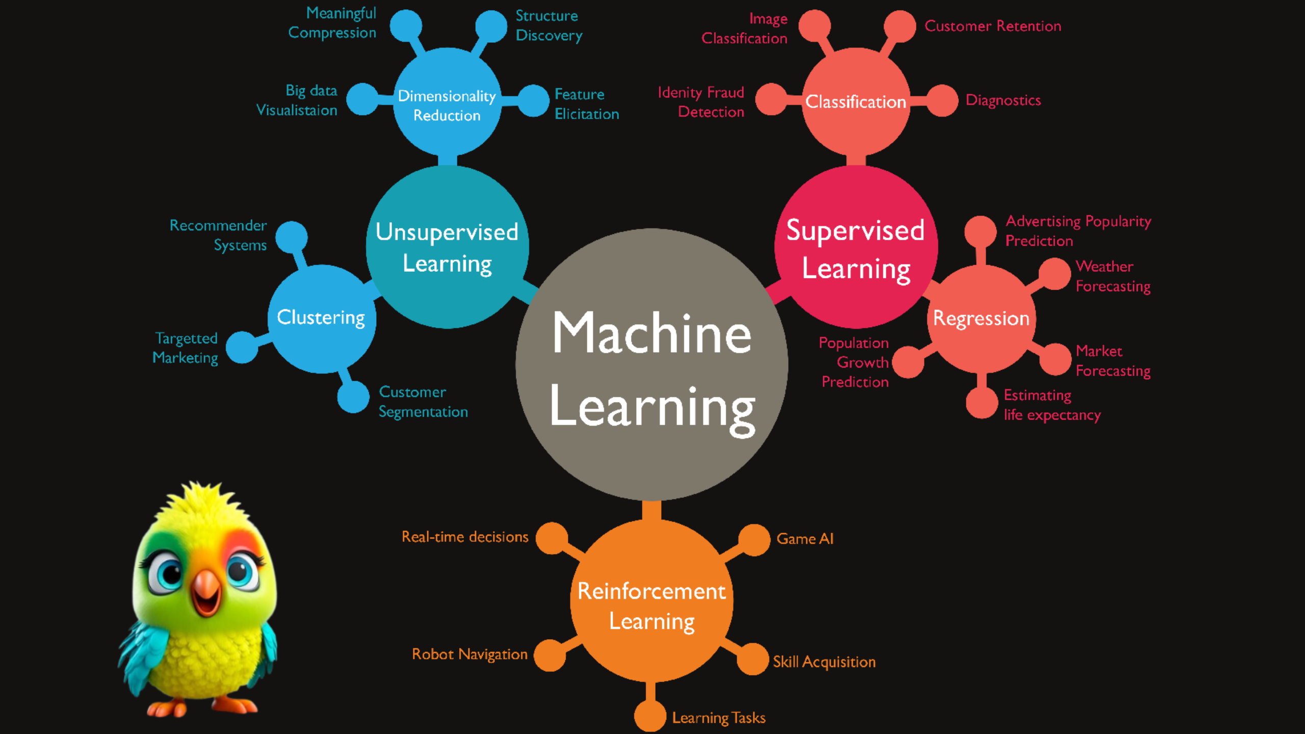
Artificial intelligence vs machine learning vs deep learning
Artificial intelligence, machine learning, and deep learning are often used synonymously when discussing all things AI. While the terms are correlated, they are not interchangeable.
Whereas AI is a broad field, machine learning is an application of AI that allows machines to learn without being specifically programmed. Machine learning is more explicitly used as a means to extract knowledge from data through simpler methods such as decision trees or linear regression, while deep learning uses the more advanced methods found in artificial neural networks.
Deep learning requires less human intervention, as features of a dataset are extracted automatically, versus simpler machine learning techniques that often require an engineer to manually identify features and classifiers of the data and adjust the algorithm accordingly. Essentially, deep learning can learn from its own errors while machine learning needs a human to intervene.
Deep learning also requires much more data than machine learning, which in turn requires significantly more computational power. Machine learning can typically be done with servers running CPUs, while deep learning often requires more robust chips such as GPUs.
Machine learning(ML) is one of the hottest buzzwords in the tech world that involves teaching machines to learn and improve from experience without being explicitly programmed. It’s like a way for machines to learn and adapt on their own, much like we as humans learn from our life experiences. ML has dramatically changed our lives by automating tasks that humans used to complete – taking up a lot of time, effort, and money from us.
What is machine learning in general?
Machine learning is a subset of artificial intelligence that enables computers to learn and improve from experience without being explicitly programmed. Unlike traditional programming, where a programmer writes code to perform a specific task, in machine learning, the system uses statistical algorithms to analyze data and improve its performance over time.
Deep learning vs. machine learning
Machine learning is a subset of artificial intelligence. In turn, deep learning is a subset of machine learning. Essentially, all deep learning is machine learning, and all machine learning is artificial intelligence, but not all artificial intelligence is machine learning.
What is deep learning?
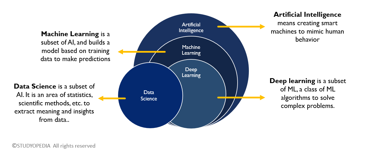
Deep learning is a subset of machine learning that uses artificial neural networks to process and analyze information. Neural networks are composed of computational nodes that are layered within deep learning algorithms. Each layer contains an input layer, an output layer, and a hidden layer. The neural network is fed training data which helps the algorithm learn and improve accuracy. When a neural network is composed of three or more layers it is said to be “deep,” thus deep learning.
Deep learning algorithms are inspired by the workings of the human brain and are used for analysis of data with a logical structure. Deep learning is used in many of the tasks we think of as AI today, including image and speech recognition, object detection, and natural language processing. Deep learning can make non-linear, complex correlations within datasets though requires more training data and computational resources than machine learning.
Mathematics behind each neuron is represented as below:

Here’s a clean, step-by-step breakdown of the mathematical operations inside a single neuron, stripped of all non-mathematical content:
1. Weighted Sum (Net Input)
$$
z = \sum_{i=1}^n w_i x_i + b
$$
– $x_i$: Input features
– $w_i$: Weights
– $b$: Bias term
2. Activation Function
$$
a = \phi(z)
$$
Common activations:
– Sigmoid:
$$\phi(z) = \frac{1}{1 + e^{-z}}$$
– ReLU:
$$\phi(z) = \max(0, z)$$
– Tanh:
$$\phi(z) = \tanh(z)$$
3. Error Calculation (Output Layer)
For a target $t$ and predicted output $y = a^{(L)}$ (where $L$ is the output layer):
$$
\delta^{(L)} = (y – t) \odot \phi'(z^{(L)})
$$
– $\odot$: Element-wise multiplication
– $\phi’$: Derivative of the activation function
4. Backpropagation (Hidden Layers)
For layer $l$:
$$
\delta^{(l)} = \left( (W^{(l+1)})^T \delta^{(l+1)} \right) \odot \phi'(z^{(l)})
$$
– $W^{(l+1)}$: Weight matrix of the next layer
5. Weight Update (Gradient Descent)
$$
w_{ij} \leftarrow w_{ij} – \eta \, \delta_j^{(l)} \, a_i^{(l-1)}
$$
$$
b_j \leftarrow b_j – \eta \, \delta_j^{(l)}
$$
– $\eta$: Learning rate
6. Summary of Steps
1. Forward Pass:
$$z = Wx + b \quad \rightarrow \quad a = \phi(z)$$
2. Backward Pass:
$$\delta = \text{Error} \odot \phi'(z)$$
3. Update:
$$W \leftarrow W – \eta \, \delta \, a^\top$$
$$b \leftarrow b – \eta \, \delta$$
This is the core mathematical flow of a neuron during training.
Here’s a step-by-step derivation of all key equations in a neural network neuron, from forward propagation to backpropagation, with mathematical rigor:
1. Forward Propagation (Expanded)
Weighted Sum:
$$
z_j = \sum_{i=1}^n w_{ji} x_i + b_j
$$
– Derivation:
Each input \(x_i\) is multiplied by its corresponding weight \(w_{ji}\), and the bias \(b_j\) is added. This is a linear transformation.
Activation Function:
$$
a_j = \phi(z_j)
$$
– Derivative Examples:
– Sigmoid:
$$\phi'(z_j) = \phi(z_j)(1 – \phi(z_j))$$
– ReLU:
$$\phi'(z_j) = \begin{cases}
1 & \text{if } z_j > 0 \\
0 & \text{otherwise}
\end{cases}$$
– Tanh:
$$\phi'(z_j) = 1 – \tanh^2(z_j)$$
2. Backpropagation (Derivation)
Output Layer Error:
For loss function \( \mathcal{L} \) (e.g., Mean Squared Error):
$$
\delta_j^{(L)} = \frac{\partial \mathcal{L}}{\partial z_j^{(L)}}
$$
– Derivation for MSE (\(\mathcal{L} = \frac{1}{2}(y_j – t_j)^2\)):
$$
\delta_j^{(L)} = \underbrace{(y_j – t_j)}_{\text{Loss gradient}} \cdot \underbrace{\phi'(z_j^{(L)})}_{\text{Activation gradient}}
$$
Hidden Layer Error:
$$
\delta_j^{(l)} = \sum_k \left( \delta_k^{(l+1)} w_{kj}^{(l+1)} \right) \phi'(z_j^{(l)})
$$
– Derivation:
Uses the chain rule to propagate error backward:
$$
\frac{\partial \mathcal{L}}{\partial z_j^{(l)}} = \sum_k \frac{\partial \mathcal{L}}{\partial z_k^{(l+1)}} \cdot \frac{\partial z_k^{(l+1)}}{\partial a_j^{(l)}} \cdot \frac{\partial a_j^{(l)}}{\partial z_j^{(l)}}
$$
– \(\frac{\partial z_k^{(l+1)}}{\partial a_j^{(l)}} = w_{kj}^{(l+1)}\) (weight linking neuron \(j\) to \(k\))
– \(\frac{\partial a_j^{(l)}}{\partial z_j^{(l)}} = \phi'(z_j^{(l)})\)
3. Weight/Bias Update (Derivation)
Gradient Descent Rule:
$$
\frac{\partial \mathcal{L}}{\partial w_{ji}^{(l)}} = \delta_j^{(l)} a_i^{(l-1)}
$$
$$
\frac{\partial \mathcal{L}}{\partial b_j^{(l)}} = \delta_j^{(l)}
$$
– Derivation:
– From \(z_j^{(l)} = \sum_i w_{ji}^{(l)} a_i^{(l-1)} + b_j^{(l)}\):
– \(\frac{\partial z_j^{(l)}}{\partial w_{ji}^{(l)}} = a_i^{(l-1)}\)
– \(\frac{\partial z_j^{(l)}}{\partial b_j^{(l)}} = 1\)
– Apply chain rule:
$$
\frac{\partial \mathcal{L}}{\partial w_{ji}^{(l)}} = \underbrace{\frac{\partial \mathcal{L}}{\partial z_j^{(l)}}}_{\delta_j^{(l)}} \cdot \frac{\partial z_j^{(l)}}{\partial w_{ji}^{(l)}}
$$
Update Equations:
$$
w_{ji}^{(l)} \leftarrow w_{ji}^{(l)} – \eta \frac{\partial \mathcal{L}}{\partial w_{ji}^{(l)}}
$$
$$
b_j^{(l)} \leftarrow b_j^{(l)} – \eta \frac{\partial \mathcal{L}}{\partial b_j^{(l)}}
$$
4. Full Algorithm Summary
1. Forward Pass:
– Compute \(z_j^{(l)} = W^{(l)} a^{(l-1)} + b^{(l)}\)
– Apply activation: \(a_j^{(l)} = \phi(z_j^{(l)})\)
2. Backward Pass:
– Output layer:
$$\delta^{(L)} = \nabla_a \mathcal{L} \odot \phi'(z^{(L)})$$
– Hidden layers (\(l = L-1, \dots, 1\)):
$$\delta^{(l)} = (W^{(l+1)})^\top \delta^{(l+1)} \odot \phi'(z^{(l)})$$
3. Update Parameters:
– \(\Delta W^{(l)} = -\eta \, \delta^{(l)} (a^{(l-1)})^\top\)
– \(\Delta b^{(l)} = -\eta \, \delta^{(l)}\)
Key Insights:
– Chain Rule: Backpropagation is just repeated application of the chain rule.
– Locality: Each neuron only needs its own \(z_j\), \(a_j\), and \(\delta_j\) to compute updates.
– Modularity: Change \(\phi\) or \(\mathcal{L}\) by plugging in different derivatives.
Here’s a complete numerical example of a neural network forward/backward pass with concrete numbers, using a single data point:
Network Architecture
– Inputs: \( x = [2.0, 3.0] \)
– Weights: \( W = \begin{bmatrix} 0.5 & -1.2 \\ 0.8 & 0.7 \end{bmatrix} \) (Layer 1)
– Bias: \( b = [0.1, -0.3] \)
– Activation: Sigmoid (\( \phi(z) = \frac{1}{1+e^{-z}} \))
– Target: \( t = 1.0 \) (binary classification)
Step 1: Forward Pass
1. Weighted Sum (\( z = Wx + b \)):
\[
z_1 = (0.5 \times 2.0) + (-1.2 \times 3.0) + 0.1 = -2.5
\]
\[
z_2 = (0.8 \times 2.0) + (0.7 \times 3.0) + (-0.3) = 3.0
\]
– Output: \( z = [-2.5, 3.0] \)
2. Activation (\( a = \phi(z) \)):
\[
a_1 = \frac{1}{1+e^{2.5}} \approx 0.076
\]
\[
a_2 = \frac{1}{1+e^{-3.0}} \approx 0.953
\]
– Activated Output: \( a = [0.076, 0.953] \)
Step 2: Output Layer Error (Binary Cross-Entropy Loss)
– Predicted Probability: \( y = a_2 = 0.953 \)
– Error Gradient (\( \delta^{(L)} = y – t \)):
\[
\delta^{(L)} = 0.953 – 1.0 = -0.047
\]
Step 3: Backpropagation (Hidden Layer)
1. Weight Gradient (\( \nabla W = \delta \cdot a^\top \)):
\[
\nabla W_{21} = \delta^{(L)} \times a_1 = -0.047 \times 0.076 \approx -0.0036
\]
\[
\nabla W_{22} = \delta^{(L)} \times a_2 = -0.047 \times 0.953 \approx -0.0448
\]
2. Bias Gradient (\( \nabla b = \delta \)):
\[
\nabla b_2 = -0.047
\]
Step 4: Update Weights (Learning Rate \( \eta = 0.1 \))
– New Weights:
\[
W_{21} \leftarrow 0.8 – (0.1 \times -0.0036) \approx 0.8004
\]
\[
W_{22} \leftarrow 0.7 – (0.1 \times -0.0448) \approx 0.7045
\]
– New Bias:
\[
b_2 \leftarrow -0.3 – (0.1 \times -0.047) \approx -0.2953
\]
Key Observations
1. Forward Pass:
– Input \( [2.0, 3.0] \) → Activated output \( \approx 0.953 \).
2. Backward Pass:
– Small error (\( -0.047 \)) slightly adjusts weights toward the target \( 1.0 \).
3. Sigmoid Behavior:
– \( z_1 = -2.5 \) → Near \( 0 \) (inactive neuron).
– \( z_2 = 3.0 \) → Near \( 1 \) (active neuron).
Why This Matters
– Transparency: Every number is traceable to show how gradients flow.
– Debugging: Verify your implementation matches these exact values.
Some common types of neural networks used for deep learning include:
Feedforward neural networks (FF) are one of the oldest forms of neural networks, with data flowing one way through layers of artificial neurons until the output is achieved.
Training a Feedforward Neural Network
Training a Feedforward Neural Network involves adjusting the weights of the neurons to minimize the error between the predicted output and the actual output. This process is typically performed using backpropagation and gradient descent.
- Forward Propagation: During forward propagation the input data passes through the network and the output is calculated.
- Loss Calculation: The loss (or error) is calculated using a loss function such as Mean Squared Error (MSE) for regression tasks or Cross-Entropy Loss for classification tasks.
- Backpropagation: In backpropagation the error is propagated back through the network to update the weights. The gradient of the loss function with respect to each weight is calculated and the weights are adjusted using gradient descent.
Evaluation of Feedforward neural network
Evaluating the performance of the trained model involves several metrics:
- Accuracy: The proportion of correctly classified instances out of the total instances.
- Precision: The ratio of true positive predictions to the total predicted positives.
- Recall: The ratio of true positive predictions to the actual positives.
- F1 Score: The harmonic mean of precision and recall, providing a balance between the two.
- Confusion Matrix: A table used to describe the performance of a classification model, showing the true positives, true negatives, false positives, and false negatives.
Code Implementation of Feedforward neural network
Model is compiled with the Adam optimizer, SparseCategoricalCrossentropy loss function and SparseCategoricalAccuracy metric and then trained for 5 epochs on the training data.
1 2 3 4 5 6 7 8 9 10 11 12 13 14 15 16 17 18 19 20 21 22 23 24 25 26 27 28 29 30 31 32 | import tensorflow as tf from tensorflow.keras.models import Sequential from tensorflow.keras.layers import Dense, Flatten from tensorflow.keras.optimizers import Adam from tensorflow.keras.losses import SparseCategoricalCrossentropy from tensorflow.keras.metrics import SparseCategoricalAccuracy # Load and prepare the MNIST dataset mnist = tf.keras.datasets.mnist (x_train, y_train), (x_test, y_test) = mnist.load_data() x_train, x_test = x_train / 255.0, x_test / 255.0 # Build the model model = Sequential([ Flatten(input_shape=(28, 28)), Dense(128, activation='relu'), Dense(10, activation='softmax') ]) # Compile the model model.compile(optimizer=Adam(), loss=SparseCategoricalCrossentropy(), metrics=[SparseCategoricalAccuracy()]) # Train the model model.fit(x_train, y_train, epochs=5) # Evaluate the model test_loss, test_acc = model.evaluate(x_test, y_test) print(f'\nTest accuracy: {test_acc}') |
This code demonstrates the process of building, training and evaluating a neural network model using TensorFlow and Keras to classify handwritten digits from the MNIST dataset.
The model architecture is defined using the Sequential API consisting of:
- a Flatten layer to convert the 2D image input into a 1D array
- a Dense layer with 128 neurons and ReLU activation
- a final Dense layer with 10 neurons and softmax activation to output probabilities for each digit class.
An epoch is when all the training data is used at once and is defined as the total number of iterations of all the training data in one cycle for training the machine learning model.
Recurrent neural networks (RNN) differ from feedforward neural networks in that they typically use time series data or data that involves sequences. Recurrent neural networks have “memory” of what happened in the previous layer as contingent to the output of the current layer.
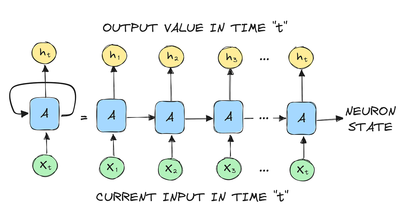
Imagine reading a sentence and you try to predict the next word, you don’t rely only on the current word but also remember the words that came before. RNNs work similarly by “remembering” past information and passing the output from one step as input to the next i.e it considers all the earlier words to choose the most likely next word. This memory of previous steps helps the network understand context and make better predictions.
Key Components of RNNs
There are mainly two components of RNNs that we will discuss.
1. Recurrent Neurons
The fundamental processing unit in RNN is a Recurrent Unit. They hold a hidden state that maintains information about previous inputs in a sequence. Recurrent units can “remember” information from prior steps by feeding back their hidden state, allowing them to capture dependencies across time.
![4. Recurrent Neural Networks - Neural networks and deep learning [Book]](https://kncmap.com/wp-content/uploads/2025/06/mlst_1401.png)
2. RNN Unfolding
RNN unfolding or unrolling is the process of expanding the recurrent structure over time steps. During unfolding each step of the sequence is represented as a separate layer in a series illustrating how information flows across each time step.
This unrolling enables backpropagation through time (BPTT) a learning process where errors are propagated across time steps to adjust the network’s weights enhancing the RNN’s ability to learn dependencies within sequential data.
Types Of Recurrent Neural Networks
There are four types of RNNs based on the number of inputs and outputs in the network:
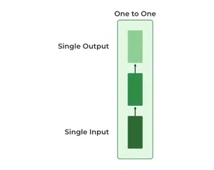
1. One-to-One RNN
This is the simplest type of neural network architecture where there is a single input and a single output. It is used for straightforward classification tasks such as binary classification where no sequential data is involved.
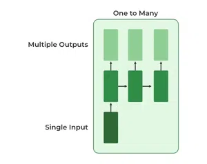
2. One-to-Many RNN
In a One-to-Many RNN the network processes a single input to produce multiple outputs over time. This is useful in tasks where one input triggers a sequence of predictions (outputs). For example in image captioning a single image can be used as input to generate a sequence of words as a caption.
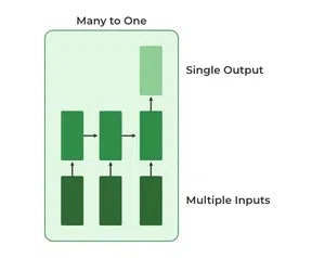
3. Many-to-One RNN
The Many-to-One RNN receives a sequence of inputs and generates a single output. This type is useful when the overall context of the input sequence is needed to make one prediction. In sentiment analysis the model receives a sequence of words (like a sentence) and produces a single output like positive, negative or neutral.
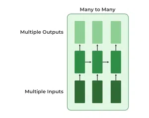
4. Many-to-Many RNN
The Many-to-Many RNN type processes a sequence of inputs and generates a sequence of outputs. In language translation task a sequence of words in one language is given as input and a corresponding sequence in another language is generated as output.
Variants of Recurrent Neural Networks (RNNs)
There are several variations of RNNs, each designed to address specific challenges or optimize for certain tasks:
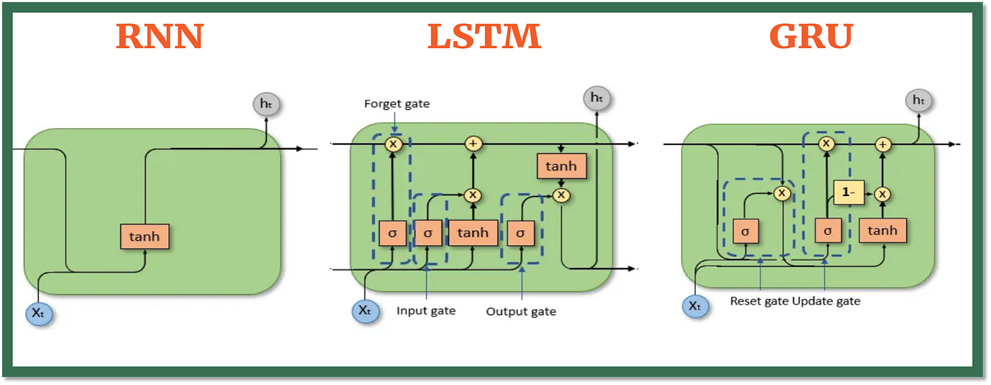
1. Vanilla RNN
This simplest form of RNN consists of a single hidden layer where weights are shared across time steps. Vanilla RNNs are suitable for learning short-term dependencies but are limited by the vanishing gradient problem, which hampers long-sequence learning.
2. Bidirectional RNNs
Bidirectional RNNs process inputs in both forward and backward directions, capturing both past and future context for each time step. This architecture is ideal for tasks where the entire sequence is available, such as named entity recognition and question answering.
3. Long Short-Term Memory Networks (LSTMs)
Long Short-Term Memory Networks (LSTMs) introduce a memory mechanism to overcome the vanishing gradient problem. Each LSTM cell has three gates:
- Input Gate: Controls how much new information should be added to the cell state.
- Forget Gate: Decides what past information should be discarded.
- Output Gate: Regulates what information should be output at the current step. This selective memory enables LSTMs to handle long-term dependencies, making them ideal for tasks where earlier context is critical.
4. Gated Recurrent Units (GRUs)
Gated Recurrent Units (GRUs) simplify LSTMs by combining the input and forget gates into a single update gate and streamlining the output mechanism. This design is computationally efficient, often performing similarly to LSTMs and is useful in tasks where simplicity and faster training are beneficial.
Long/short term memory (LSTM) is an advanced form of RNN that can use memory to “remember” what happened in previous layers.
LSTMs can capture long-term dependencies in sequential data making them ideal for tasks like language translation, speech recognition and time series forecasting.
Unlike traditional RNNs which use a single hidden state passed through time LSTMs introduce a memory cell that holds information over extended periods addressing the challenge of learning long-term dependencies.
Applications of LSTM
Some of the famous applications of LSTM includes:
- Language Modeling: Used in tasks like language modeling, machine translation and text summarization. These networks learn the dependencies between words in a sentence to generate coherent and grammatically correct sentences.
- Speech Recognition: Used in transcribing speech to text and recognizing spoken commands. By learning speech patterns they can match spoken words to corresponding text.
- Time Series Forecasting: Used for predicting stock prices, weather and energy consumption. They learn patterns in time series data to predict future events.
- Anomaly Detection: Used for detecting fraud or network intrusions. These networks can identify patterns in data that deviate drastically and flag them as potential anomalies.
- Recommender Systems: In recommendation tasks like suggesting movies, music and books. They learn user behavior patterns to provide personalized suggestions.
- Video Analysis: Applied in tasks such as object detection, activity recognition and action classification. When combined with Convolutional Neural Networks (CNNs) they help analyze video data and extract useful information.
Convolutional neural networks (CNN) include some of the most common neural networks in modern artificial intelligence and use several distinct layers (a convolutional layer, then a pooling layer) that filter different parts of an image before putting it back together (in the fully connected layer).
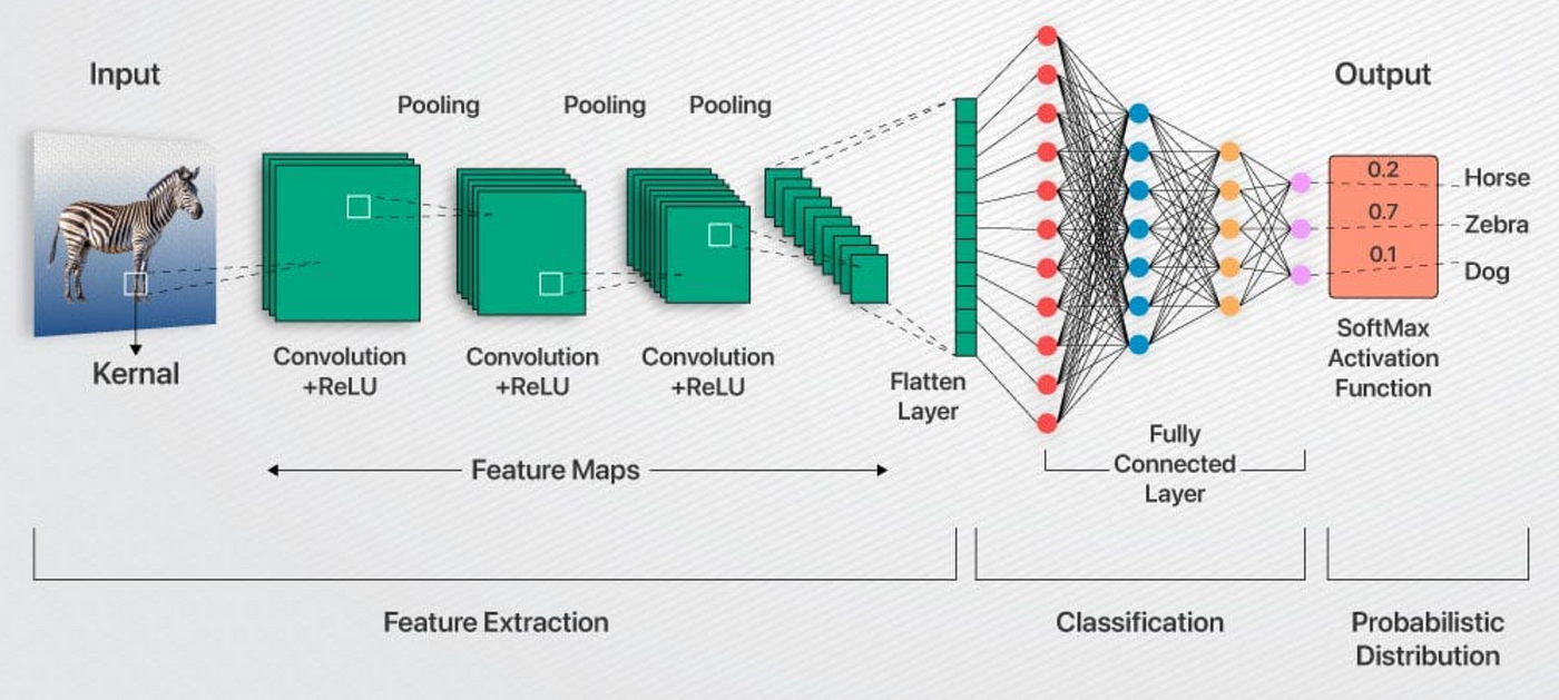
This is particularly useful for visual datasets such as images or videos, where data patterns play a crucial role. CNNs are widely used in computer vision applications due to their effectiveness in processing visual data.
CNNs consist of multiple layers like the input layer, Convolutional layer, pooling layer, and fully connected layers.
How Convolutional Layers Works?
Convolution Neural Networks are neural networks that share their parameters.
Imagine you have an image. It can be represented as a cuboid having its length, width (dimension of the image), and height (i.e the channel as images generally have red, green, and blue channels).
Now imagine taking a small patch of this image and running a small neural network, called a filter or kernel on it, with say, K outputs and representing them vertically.
Now slide that neural network across the whole image, as a result, we will get another image with different widths, heights, and depths. Instead of just R, G, and B channels now we have more channels but lesser width and height. This operation is called Convolution. If the patch size is the same as that of the image it will be a regular neural network. Because of this small patch, we have fewer weights.
Mathematical Overview of Convolution
Now let’s talk about a bit of mathematics that is involved in the whole convolution process.
- Convolution layers consist of a set of learnable filters (or kernels) having small widths and heights and the same depth as that of input volume (3 if the input layer is image input).
- For example, if we have to run convolution on an image with dimensions 34x34x3. The possible size of filters can be axax3, where ‘a’ can be anything like 3, 5, or 7 but smaller as compared to the image dimension.
- During the forward pass, we slide each filter across the whole input volume step by step where each step is called stride (which can have a value of 2, 3, or even 4 for high-dimensional images) and compute the dot product between the kernel weights and patch from input volume.
- As we slide our filters we’ll get a 2-D output for each filter and we’ll stack them together as a result, we’ll get output volume having a depth equal to the number of filters. The network will learn all the filters.
Layers Used to Build ConvNets
A complete Convolution Neural Networks architecture is also known as covnets. A covnets is a sequence of layers, and every layer transforms one volume to another through a differentiable function.
Let’s take an example by running a covnets on of image of dimension 32 x 32 x 3.
- Input Layers: It’s the layer in which we give input to our model. In CNN, Generally, the input will be an image or a sequence of images. This layer holds the raw input of the image with width 32, height 32, and depth 3.
- Convolutional Layers: This is the layer, which is used to extract the feature from the input dataset. It applies a set of learnable filters known as the kernels to the input images. The filters/kernels are smaller matrices usually 2×2, 3×3, or 5×5 shape. it slides over the input image data and computes the dot product between kernel weight and the corresponding input image patch. The output of this layer is referred as feature maps. Suppose we use a total of 12 filters for this layer we’ll get an output volume of dimension 32 x 32 x 12.
- Activation Layer: By adding an activation function to the output of the preceding layer, activation layers add nonlinearity to the network. it will apply an element-wise activation function to the output of the convolution layer. Some common activation functions are RELU: max(0, x), Tanh, Leaky RELU, etc. The volume remains unchanged hence output volume will have dimensions 32 x 32 x 12.
- Pooling layer: This layer is periodically inserted in the covnets and its main function is to reduce the size of volume which makes the computation fast reduces memory and also prevents overfitting. Two common types of pooling layers are max pooling and average pooling. If we use a max pool with 2 x 2 filters and stride 2, the resultant volume will be of dimension 16x16x12.
- Flattening: The resulting feature maps are flattened into a one-dimensional vector after the convolution and pooling layers so they can be passed into a completely linked layer for categorization or regression.
- Fully Connected Layers: It takes the input from the previous layer and computes the final classification or regression task.
- Output Layer: The output from the fully connected layers is then fed into a logistic function for classification tasks like sigmoid or softmax which converts the output of each class into the probability score of each class.
Example: Applying CNN to an Image
Let’s consider an image and apply the convolution layer, activation layer, and pooling layer operation to extract the inside feature.
Input image:

Step:
- import the necessary libraries
- set the parameter
- define the kernel
- Load the image and plot it.
- Reformat the image
- Apply convolution layer operation and plot the output image.
- Apply activation layer operation and plot the output image.
- Apply pooling layer operation and plot the output image.
NOTE: AM USING COLAB
1 2 3 4 5 6 7 8 9 10 11 12 13 14 15 16 17 18 19 20 21 22 23 24 25 26 27 28 29 30 31 32 33 34 35 36 37 38 39 40 41 42 43 44 45 46 47 48 49 50 51 52 53 54 55 56 57 58 59 60 61 62 63 64 65 66 67 68 69 70 71 72 73 74 75 76 77 78 79 80 81 82 83 84 85 86 87 | # import the necessary libraries import numpy as np import tensorflow as tf import matplotlib.pyplot as plt from itertools import product # set the param plt.rc('figure', autolayout=True) plt.rc('image', cmap='magma') # define the kernel kernel = tf.constant([[-1, -1, -1], [-1, 8, -1], [-1, -1, -1], ]) # load the image image = tf.io.read_file('/content/Ganesh.jpg') image = tf.io.decode_jpeg(image, channels=1) image = tf.image.resize(image, size=[300, 300]) # plot the image img = tf.squeeze(image).numpy() plt.figure(figsize=(5, 5)) plt.imshow(img, cmap='gray') plt.axis('off') plt.title('Original Gray Scale image') plt.show(); # Reformat image = tf.image.convert_image_dtype(image, dtype=tf.float32) image = tf.expand_dims(image, axis=0) kernel = tf.reshape(kernel, [*kernel.shape, 1, 1]) kernel = tf.cast(kernel, dtype=tf.float32) # convolution layer conv_fn = tf.nn.conv2d image_filter = conv_fn( input=image, filters=kernel, strides=1, # or (1, 1) padding='SAME', ) plt.figure(figsize=(15, 5)) # Plot the convolved image plt.subplot(1, 3, 1) plt.imshow( tf.squeeze(image_filter) ) plt.axis('off') plt.title('Convolution') # activation layer relu_fn = tf.nn.relu # Image detection image_detect = relu_fn(image_filter) plt.subplot(1, 3, 2) plt.imshow( # Reformat for plotting tf.squeeze(image_detect) ) plt.axis('off') plt.title('Activation') # Pooling layer pool = tf.nn.pool image_condense = pool(input=image_detect, window_shape=(2, 2), pooling_type='MAX', strides=(2, 2), padding='SAME', ) plt.subplot(1, 3, 3) plt.imshow(tf.squeeze(image_condense)) plt.axis('off') plt.title('Pooling') plt.show() |
OUTPUT:
Advantages of CNNs
- Good at detecting patterns and features in images, videos, and audio signals.
- Robust to translation, rotation, and scaling invariance.
- End-to-end training, no need for manual feature extraction.
- Can handle large amounts of data and achieve high accuracy.
Disadvantages of CNNs
- Computationally expensive to train and require a lot of memory.
- Can be prone to overfitting if not enough data or proper regularization is used.
- Requires large amounts of labeled data.
- Interpretability is limited, it’s hard to understand what the network has learned.
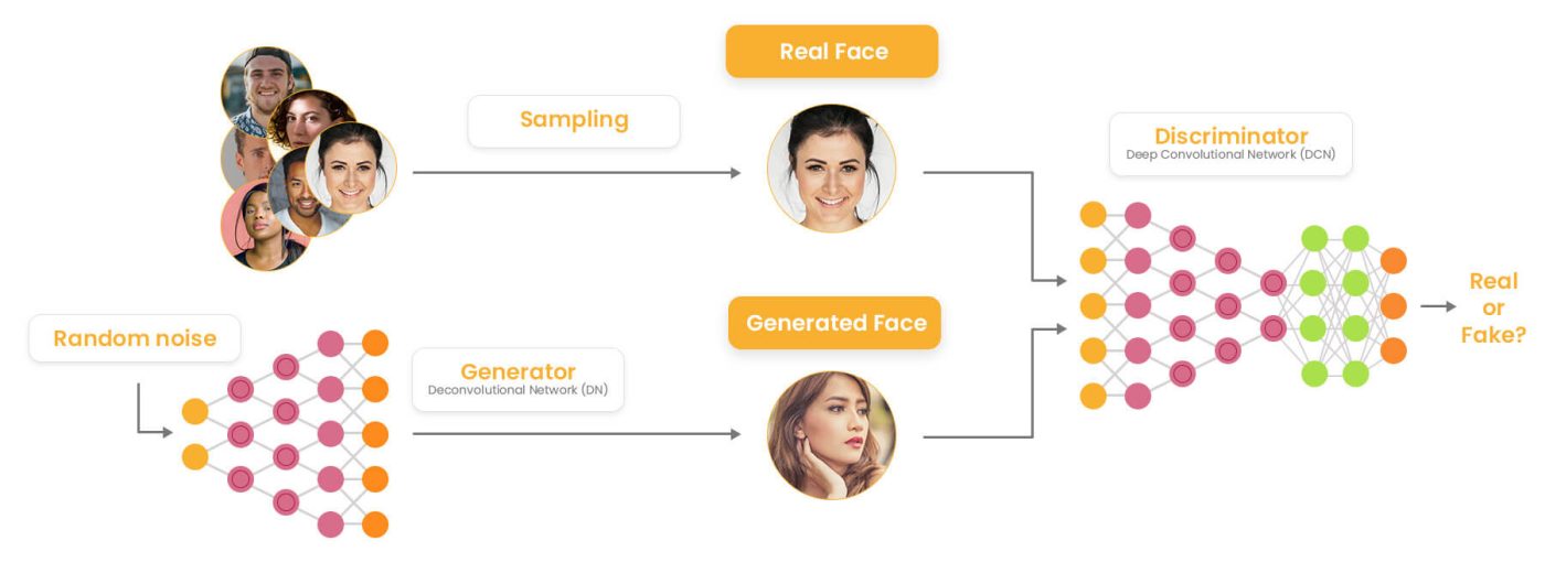
Generative adversarial networks (GAN) involve two neural networks (a “generator” and a “discriminator”) that compete against each other in a game that ultimately improves the accuracy of the output. It is introduced by Ian Goodfellow and his team in 2014 and they have transformed how computers generate images, videos, music and more. Unlike traditional models that only recognize or classify data, they take a creative way by generating entirely new content that closely resembles real-world data. This ability helped various fields such as art, gaming, healthcare and data science. In this article, we will see more about GANs and its core concepts.
Architecture of GANs
GANs consist of two main models that work together to create realistic synthetic data which are as follows:
1. Generator Model
The generator is a deep neural network that takes random noise as input to generate realistic data samples like images or text. It learns the underlying data patterns by adjusting its internal parameters during training through backpropagation. Its objective is to produce samples that the discriminator classifies as real.
How does a GAN work?
GANs train by having two networks the Generator (G) and the Discriminator (D) compete and improve together. Here’s the step-by-step process
1. Generator’s First Move
The generator starts with a random noise vector like random numbers. It uses this noise as a starting point to create a fake data sample such as a generated image. The generator’s internal layers transform this noise into something that looks like real data.
2. Discriminator’s Turn
The discriminator receives two types of data:
- Real samples from the actual training dataset.
- Fake samples created by the generator.
D’s job is to analyze each input and find whether it’s real data or something G cooked up. It outputs a probability score between 0 and 1. A score of 1 shows the data is likely real and 0 suggests it’s fake.
3. Adversarial Learning
- If the discriminator correctly classifies real and fake data it gets better at its job.
- If the generator fools the discriminator by creating realistic fake data, it receives a positive update and the discriminator is penalized for making a wrong decision.
4. Generator’s Improvement
- Each time the discriminator mistakes fake data for real, the generator learns from this success.
- Through many iterations, the generator improves and creates more convincing fake samples.
5. Discriminator’s Adaptation
- The discriminator also learns continuously by updating itself to better spot fake data.
- This constant back-and-forth makes both networks stronger over time.
6. Training Progression
- As training continues, the generator becomes highly proficient at producing realistic data.
- Eventually the discriminator struggles to distinguish real from fake shows that the GAN has reached a well-trained state.
- At this point, the generator can produce high-quality synthetic data that can be used for different applications.
Types of GANs

There are several types of GANs each designed for different purposes. Here are some important types:
1. Vanilla GAN
Vanilla GAN is the simplest type of GAN. It consists of:
- A generator and a discriminator both are built using multi-layer perceptrons (MLPs).
- The model optimizes its mathematical formulation using stochastic gradient descent (SGD).
While foundational, Vanilla GANs can face problems like:
- Mode collapse: The generator produces limited types of outputs repeatedly.
- Unstable training: The generator and discriminator may not improve smoothly.
2. Conditional GAN (CGAN)
Conditional GANs (CGANs) adds an additional conditional parameter to guide the generation process. Instead of generating data randomly they allow the model to produce specific types of outputs.
Working of CGANs:
- A conditional variable (y) is fed into both the generator and the discriminator.
- This ensures that the generator creates data corresponding to the given condition (e.g generating images of specific objects).
- The discriminator also receives the labels to help distinguish between real and fake data.
Example: Instead of generating any random image, CGAN can generate a specific object like a dog or a cat based on the label.
3. Deep Convolutional GAN (DCGAN)
Deep Convolutional GANs (DCGANs) are among the most popular types of GANs used for image generation.
They are important because they:
- Uses Convolutional Neural Networks (CNNs) instead of simple multi-layer perceptrons (MLPs).
- Max pooling layers are replaced with convolutional stride helps in making the model more efficient.
- Fully connected layers are removed, which allows for better spatial understanding of images.
DCGANs are successful because they generate high-quality, realistic images.
4. Laplacian Pyramid GAN (LAPGAN)
Laplacian Pyramid GAN (LAPGAN) is designed to generate ultra-high-quality images by using a multi-resolution approach.
Working of LAPGAN:
- Uses multiple generator-discriminator pairs at different levels of the Laplacian pyramid.
- Images are first down sampled at each layer of the pyramid and upscaled again using Conditional GANs (CGANs).
- This process allows the image to gradually refine details and helps in reducing noise and improving clarity.
Due to its ability to generate highly detailed images, LAPGAN is considered a superior approach for photorealistic image generation.
5. Super Resolution GAN (SRGAN)
Super-Resolution GAN (SRGAN) is designed to increase the resolution of low-quality images while preserving details.
Working of SRGAN:
- Uses a deep neural network combined with an adversarial loss function.
- Enhances low-resolution images by adding finer details helps in making them appear sharper and more realistic.
- Helps to reduce common image upscaling errors such as blurriness and pixelation.
Implementation of Generative Adversarial Network (GAN) using PyTorch
Generative Adversarial Networks (GANs) can generate realistic images by learning from existing image datasets. Here we will be implementing a GAN trained on the CIFAR-10 dataset using PyTorch.
Step 1: Importing Required Libraries
We will be using Pytorch, Torchvision, Matplotlib and Numpy libraries for this. Set the device to GPU if available otherwise use CPU.
Dataset: https://www.cs.toronto.edu/~kriz/cifar-10-python.tar.gz or https://www.cs.toronto.edu/~kriz/cifar.html
1 2 3 4 5 6 7 8 9 10 11 12 13 14 15 16 17 18 19 20 21 22 23 24 25 26 27 28 29 30 31 32 33 34 35 36 37 38 39 40 41 42 43 44 45 46 47 48 49 50 51 52 53 54 55 56 57 58 59 60 61 62 63 64 65 66 67 68 69 70 71 72 73 74 75 76 77 78 79 80 81 82 83 84 85 86 87 88 89 90 91 92 93 94 95 96 97 98 99 100 101 102 103 104 105 106 107 108 109 110 111 112 113 114 115 116 117 118 119 120 121 122 123 124 125 126 127 128 129 130 131 132 133 134 135 136 137 138 | import torch import torch.nn as nn import torch.optim as optim import torchvision from torchvision import datasets, transforms import matplotlib.pyplot as plt import numpy as np device = torch.device('cuda' if torch.cuda.is_available() else 'cpu') transform = transforms.Compose([ transforms.ToTensor(), transforms.Normalize((0.5, 0.5, 0.5), (0.5, 0.5, 0.5)) ]) train_dataset = datasets.CIFAR10(root='./data',\ train=True, download=True, transform=transform) dataloader = torch.utils.data.DataLoader(train_dataset, \ batch_size=32, shuffle=True) latent_dim = 100 lr = 0.0002 beta1 = 0.5 beta2 = 0.999 num_epochs = 10 class Generator(nn.Module): def __init__(self, latent_dim): super(Generator, self).__init__() self.model = nn.Sequential( nn.Linear(latent_dim, 128 * 8 * 8), nn.ReLU(), nn.Unflatten(1, (128, 8, 8)), nn.Upsample(scale_factor=2), nn.Conv2d(128, 128, kernel_size=3, padding=1), nn.BatchNorm2d(128, momentum=0.78), nn.ReLU(), nn.Upsample(scale_factor=2), nn.Conv2d(128, 64, kernel_size=3, padding=1), nn.BatchNorm2d(64, momentum=0.78), nn.ReLU(), nn.Conv2d(64, 3, kernel_size=3, padding=1), nn.Tanh() ) def forward(self, z): img = self.model(z) return img class Discriminator(nn.Module): def __init__(self): super(Discriminator, self).__init__() self.model = nn.Sequential( nn.Conv2d(3, 32, kernel_size=3, stride=2, padding=1), nn.LeakyReLU(0.2), nn.Dropout(0.25), nn.Conv2d(32, 64, kernel_size=3, stride=2, padding=1), nn.ZeroPad2d((0, 1, 0, 1)), nn.BatchNorm2d(64, momentum=0.82), nn.LeakyReLU(0.25), nn.Dropout(0.25), nn.Conv2d(64, 128, kernel_size=3, stride=2, padding=1), nn.BatchNorm2d(128, momentum=0.82), nn.LeakyReLU(0.2), nn.Dropout(0.25), nn.Conv2d(128, 256, kernel_size=3, stride=1, padding=1), nn.BatchNorm2d(256, momentum=0.8), nn.LeakyReLU(0.25), nn.Dropout(0.25), nn.Flatten(), nn.Linear(256 * 5 * 5, 1), nn.Sigmoid() ) def forward(self, img): validity = self.model(img) return validity generator = Generator(latent_dim).to(device) discriminator = Discriminator().to(device) adversarial_loss = nn.BCELoss() optimizer_G = optim.Adam(generator.parameters()\ , lr=lr, betas=(beta1, beta2)) optimizer_D = optim.Adam(discriminator.parameters()\ , lr=lr, betas=(beta1, beta2)) for epoch in range(num_epochs): for i, batch in enumerate(dataloader): real_images = batch[0].to(device) valid = torch.ones(real_images.size(0), 1, device=device) fake = torch.zeros(real_images.size(0), 1, device=device) real_images = real_images.to(device) optimizer_D.zero_grad() z = torch.randn(real_images.size(0), latent_dim, device=device) fake_images = generator(z) real_loss = adversarial_loss(discriminator\ (real_images), valid) fake_loss = adversarial_loss(discriminator\ (fake_images.detach()), fake) d_loss = (real_loss + fake_loss) / 2 d_loss.backward() optimizer_D.step() optimizer_G.zero_grad() gen_images = generator(z) g_loss = adversarial_loss(discriminator(gen_images), valid) g_loss.backward() optimizer_G.step() if (i + 1) % 100 == 0: print( f"Epoch [{epoch+1}/{num_epochs}]\ Batch {i+1}/{len(dataloader)} " f"Discriminator Loss: {d_loss.item():.4f} " f"Generator Loss: {g_loss.item():.4f}" ) if (epoch + 1) % 10 == 0: with torch.no_grad(): z = torch.randn(16, latent_dim, device=device) generated = generator(z).detach().cpu() grid = torchvision.utils.make_grid(generated,\ nrow=4, normalize=True) plt.imshow(np.transpose(grid, (1, 2, 0))) plt.axis("off") plt.show() |
Application Of Generative Adversarial Networks (GANs)
- Image Synthesis & Generation: GANs generate realistic images, avatars and high-resolution visuals by learning patterns from training data. They are used in art, gaming and AI-driven design.
- Image-to-Image Translation: They can transform images between domains while preserving key features. Examples include converting day images to night, sketches to realistic images or changing artistic styles.
- Text-to-Image Synthesis: They create visuals from textual descriptions helps applications in AI-generated art, automated design and content creation.
- Data Augmentation: They generate synthetic data to improve machine learning models helps in making them more robust and generalizable in fields with limited labeled data.
- High-Resolution Image Enhancement: They upscale low-resolution images which helps in improving clarity for applications like medical imaging, satellite imagery and video enhancement.
Advantages of GAN
Lets see various advantages of the GANs:
- Synthetic Data Generation: GANs produce new, synthetic data resembling real data distributions which is useful for augmentation, anomaly detection and creative tasks.
- High-Quality Results: They can generate photorealistic images, videos, music and other media with high quality.
- Unsupervised Learning: They don’t require labeled data helps in making them effective in scenarios where labeling is expensive or difficult.
- Versatility: They can be applied across many tasks including image synthesis, text-to-image generation, style transfer, anomaly detection and more.
Supervised learning
Supervised learningis a machine learning model that uses labeled training data (structured data) to map a specific input to an output. In supervised learning, the output is known (such as recognizing a picture of an apple) and the model is trained on data of the known output. In simple terms, to train the algorithm to recognize pictures of apples, feed it pictures labeled as apples.
The most common supervised learning algorithms used today include:
- Linear regression
- Polynomial regression
- K-nearest neighbors
- Naive Bayes
- Polynomial regression
- Decision trees
Unsupervised learning
Unsupervised learning is a machine learning model that uses unlabeled data (unstructured data) to learn patterns. Unlike supervised learning, the output is not known ahead of time. Rather, the algorithm learns from the data without human input (thus, unsupervised) and categorizes it into groups based on attributes. For instance, if the algorithm is given pictures of apples and bananas, it will work by itself to categorize which picture is an apple and which is a banana. Unsupervised learning is good at descriptive modeling and pattern matching.
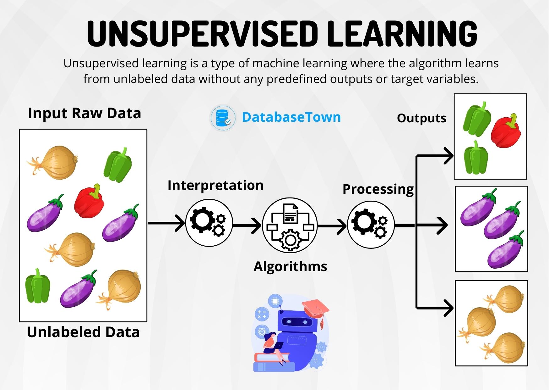
The most common unsupervised learning algorithms used today include:
- Fuzzy means
- K-means clustering
- Hierarchical clustering
- Principal component analysis
- Partial least squares
A mixed approach machine learning called semi-supervised learning is also often employed, where only some of the data is labeled. In semi-supervised learning, the algorithm must figure out how to organize and structure the data to achieve a known result. For instance, the machine learning model is told that the end result is an apple, but only some of the training data is labeled as an apple.
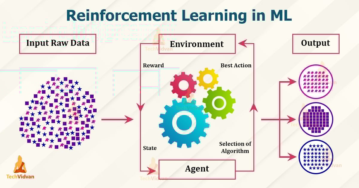
Reinforcement learning
Reinforcement learning is a machine learning model that can be described as “learn by doing” through a series of trial and error experiments. An “agent” learns to perform a defined task through a feedback loop until its performance is within a desirable range. The agent receives positive reinforcement when it performs the task well and negative reinforcement when it performs poorly. An example of reinforcement learning is when Google researchers taught a reinforcement learning algorithm to play the game Go. The model had no prior knowledge of the rules of Go and simply moved pieces at random and “learned” the best results as the algorithm was trained, to the point that the machine learning model could beat a human player at the game.
How Supervised Machine Learning Works?
Where supervised learning algorithm consists of input features and corresponding output labels. The process works through:
- Training Data: The model is provided with a training dataset that includes input data (features) and corresponding output data (labels or target variables).
- Learning Process: The algorithm processes the training data, learning the relationships between the input features and the output labels. This is achieved by adjusting the model’s parameters to minimize the difference between its predictions and the actual labels.
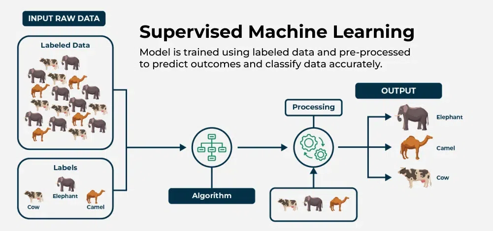
After training, the model is evaluated using a test dataset to measure its accuracy and performance. Then the model’s performance is optimized by adjusting parameters and using techniques like cross-validation to balance bias and variance. This ensures the model generalizes well to new, unseen data.
In summary, supervised machine learning involves training a model on labeled data to learn patterns and relationships, which it then uses to make accurate predictions on new data.
Let’s learn how a supervised machine learning model is trained on a dataset to learn a mapping function between input and output, and then with learned function is used to make predictions on new data:
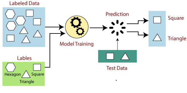
Supervised Learning Models.
Practical Examples of Supervised learning
Few practical examples of supervised machine learning across various industries:
- Fraud Detection in Banking: Utilizes supervised learning algorithms on historical transaction data, training models with labeled datasets of legitimate and fraudulent transactions to accurately predict fraud patterns.
- Parkinson Disease Prediction: Parkinson’s disease is a progressive disorder that affects the nervous system and the parts of the body controlled by the nerves.
- Customer Churn Prediction: Uses supervised learning techniques to analyze historical customer data, identifying features associated with churn rates to predict customer retention effectively.
- Cancer cell classification: Implements supervised learning for cancer cells based on their features, and identifying them if they are ‘malignant’ or ‘benign.
- Stock Price Prediction: Applies supervised learning to predict a signal that indicates whether buying a particular stock will be helpful or not.
Supervised Machine Learning Algorithms
Supervised learning can be further divided into several different types, each with its own unique characteristics and applications. Here are some of the most common types of supervised learning algorithms:
- Linear Regression: Linear regression is a type of supervised learning regression algorithm that is used to predict a continuous output value. It is one of the simplest and most widely used algorithms in supervised learning.
- Logistic Regression : Logistic regression is a type of supervised learning classification algorithm that is used to predict a binary output variable.
- Decision Trees : Decision tree is a tree-like structure that is used to model decisions and their possible consequences. Each internal node in the tree represents a decision, while each leaf node represents a possible outcome.
- Random Forests : Random forests again are made up of multiple decision trees that work together to make predictions. Each tree in the forest is trained on a different subset of the input features and data. The final prediction is made by aggregating the predictions of all the trees in the forest.
- Support Vector Machine(SVM) : The SVM algorithm creates a hyperplane to segregate n-dimensional space into classes and identify the correct category of new data points. The extreme cases that help create the hyperplane are called support vectors, hence the name Support Vector Machine.
- K-Nearest Neighbors (KNN) : KNN works by finding k training examples closest to a given input and then predicts the class or value based on the majority class or average value of these neighbors. The performance of KNN can be influenced by the choice of k and the distance metric used to measure proximity.
- Gradient Boosting : Gradient Boosting combines weak learners, like decision trees, to create a strong model. It iteratively builds new models that correct errors made by previous ones.
- Naive Bayes Algorithm: The Naive Bayes algorithm is a supervised machine learning algorithm based on applying Bayes’ Theorem with the “naive” assumption that features are independent of each other given the class label.
| Algorithm | Regression, | |||
|---|---|---|---|---|
| Classification | Purpose | Method | Use Cases | |
| Linear Regression | Regression | Predict continuous output values | Linear equation minimizing sum of squares of residuals | Predicting continuous values |
| Logistic Regression | Classification | Predict binary output variable | Logistic function transforming linear relationship | Binary classification tasks |
| Decision Trees | Both | Model decisions and outcomes | Tree-like structure with decisions and outcomes | Classification and Regression tasks |
| Random Forests | Both | Improve classification and regression accuracy | Combining multiple decision trees | Reducing overfitting, improving prediction accuracy |
| SVM | Both | Create hyperplane for classification or predict continuous values | Maximizing margin between classes or predicting continuous values | Classification and Regression tasks |
| KNN | Both | Predict class or value based on k closest neighbors | Finding k closest neighbors and predicting based on majority or average | Classification and Regression tasks, sensitive to noisy data |
| Gradient Boosting | Both | Combine weak learners to create strong model | Iteratively correcting errors with new models | Classification and Regression tasks to improve prediction accuracy |
| Naive Bayes | Classification | Predict class based on feature independence assumption | Bayes' theorem with feature independence assumption | Text classification, spam filtering, sentiment analysis, medical |
These types of supervised learning in machine learning vary based on the problem you’re trying to solve and the dataset you’re working with. In classification problems, the task is to assign inputs to predefined classes, while regression problems involve predicting numerical outcomes.
Training a Supervised Learning Model: Key Steps
The goal of Supervised learning is to generalize well to unseen data. Training a model for supervised learning involves several crucial steps, each designed to prepare the model to make accurate predictions or decisions based on labeled data. Below are the key steps involved in training a model for supervised machine learning:
- Data Collection and Preprocessing: Gather a labeled dataset consisting of input features and target output labels. Clean the data, handle missing values, and scale features as needed to ensure high quality for supervised learning algorithms.
- Splitting the Data: Divide the data into training set (80
- Choosing the Model: Select appropriate algorithms based on the problem type. This step is crucial for effective supervised learning in AI.
- Training the Model: Feed the model input data and output labels, allowing it to learn patterns by adjusting internal parameters.
- Evaluating the Model: Test the trained model on the unseen test set and assess its performance using various metrics.
- Hyperparameter Tuning: Adjust settings that control the training process (e.g., learning rate) using techniques like grid search and cross-validation.
- Final Model Selection and Testing: Retrain the model on the complete dataset using the best hyperparameters testing its performance on the test set to ensure readiness for deployment.
- Model Deployment: Deploy the validated model to make predictions on new, unseen data.
By following these steps, supervised learning models can be effectively trained to tackle various tasks, from learning a class from examples to making predictions in real-world applications.
Advantages and Disadvantages of Supervised Learning
Advantages of Supervised Learning
The power of supervised learning lies in its ability to accurately predict patterns and make data-driven decisions across a variety of applications. Here are some advantages of supervised learning listed below:
- Supervised learning excels in accurately predicting patterns and making data-driven decisions.
- Labeled training data is crucial for enabling supervised learning models to learn input-output relationships effectively.
- Supervised machine learning encompasses tasks such as supervised learning classification and supervised learning regression.
- Applications include complex problems like image recognition and natural language processing.
- Established evaluation metrics (accuracy, precision, recall, F1-score) are essential for assessing supervised learning model performance.
- Advantages of supervised learning include creating complex models for accurate predictions on new data.
- Supervised learning requires substantial labeled training data, and its effectiveness hinges on data quality and representativeness.
Disadvantages of Supervised Learning
Despite the benefits of supervised learning methods, there are notable disadvantages of supervised learning:
- Overfitting: Models can overfit training data, leading to poor performance on new data due to capturing noise in supervised machine learning.
- Feature Engineering : Extracting relevant features is crucial but can be time-consuming and requires domain expertise in supervised learning applications.
- Bias in Models: Bias in the training data may result in unfair predictions in supervised learning algorithms.
- Dependence on Labeled Data: Supervised learning relies heavily on labeled training data, which can be costly and time-consuming to obtain, posing a challenge for supervised learning techniques.
Conclusion
Supervised learning is a powerful branch of machine learning that revolves around learning a class from examples provided during training. By using supervised learning algorithms, models can be trained to make predictions based on labeled data. The effectiveness of supervised machine learning lies in its ability to generalize from the training data to new, unseen data, making it invaluable for a variety of applications, from image recognition to financial forecasting.
Understanding the types of supervised learning algorithms and the dimensions of supervised machine learning is essential for choosing the appropriate algorithm to solve specific problems. As we continue to explore the different types of supervised learning and refine these supervised learning techniques, the impact of supervised learning in machine learning will only grow, playing a critical role in advancing AI-driven solutions.
2. Unsupervised Learning
Clustering:
KMeans,DBSCAN,AgglomerativeClusteringDimensionality Reduction:
PCA,KernelPCA,TruncatedSVD,NMFManifold Learning:
TSNE,Isomap,SpectralEmbeddingMixture Models:
GaussianMixture
3. Regression:
Regression in machine learning refers to a supervised learning technique where the goal is to predict a continuous numerical value based on one or more independent features. It finds relationships between variables so that predictions can be made. we have two types of variables present in regression:
- Dependent Variable (Target): The variable we are trying to predict e.g house price.
- Independent Variables (Features): The input variables that influence the prediction e.g locality, number of rooms.
Regression analysis problem works with if output variable is a real or continuous value such as “salary” or “weight”. Many different regression models can be used but the simplest model in them is linear regression
Types of Regression
Regression can be classified into different types based on the number of predictor variables and the nature of the relationship between variables:
1. Simple Linear Regression
Linear regression is one of the simplest and most widely used statistical models. This assumes that there is a linear relationship between the independent and dependent variables. This means that the change in the dependent variable is proportional to the change in the independent variables. For example predicting the price of a house based on its size.
2. Multiple Linear Regression
Multiple linear regression extends simple linear regression by using multiple independent variables to predict target variable. For example predicting the price of a house based on multiple features such as size, location, number of rooms, etc.
3. Polynomial Regression
Polynomial regression is used to model with non-linear relationships between the dependent variable and the independent variables. It adds polynomial terms to the linear regression model to capture more complex relationships. For example when we want to predict a non-linear trend like population growth over time we use polynomial regression.
4. Ridge & Lasso Regression
Ridge & lasso regression are regularized versions of linear regression that help avoid overfitting by penalizing large coefficients. When there’s a risk of overfitting due to too many features we use these type of regression algorithms.
5. Support Vector Regression (SVR)
SVR is a type of regression algorithm that is based on the Support Vector Machine (SVM) algorithm. SVM is a type of algorithm that is used for classification tasks but it can also be used for regression tasks. SVR works by finding a hyperplane that minimizes the sum of the squared residuals between the predicted and actual values.
6. Decision Tree Regression
Decision tree Uses a tree-like structure to make decisions where each branch of tree represents a decision and leaves represent outcomes. For example predicting customer behavior based on features like age, income, etc there we use decison tree regression.
7. Random Forest Regression
Random Forest is a ensemble method that builds multiple decision trees and each tree is trained on a different subset of the training data. The final prediction is made by averaging the predictions of all of the trees. For example customer churn or sales data using this.
Regression Evaluation Metrics
Evaluation in machine learning measures the performance of a model. Here are some popular evaluation metrics for regression:
- Mean Absolute Error (MAE): The average absolute difference between the predicted and actual values of the target variable.
- Mean Squared Error (MSE): The average squared difference between the predicted and actual values of the target variable.
- Root Mean Squared Error (RMSE): Square root of the mean squared error.
- Huber Loss: A hybrid loss function that transitions from MAE to MSE for larger errors, providing balance between robustness and MSE’s sensitivity to outliers.
- R2 – Score: Higher values indicate better fit ranging from 0 to 1.
Regression Model Machine Learning
Let’s take an example of linear regression. We have a Housing data set and we want to predict the price of the house. Following is the python code for it.
1 2 3 4 5 6 7 8 9 10 11 12 13 14 15 16 17 18 19 20 21 22 23 24 25 26 27 28 29 30 31 32 33 34 35 36 37 38 39 40 41 42 | import matplotlib matplotlib.use('TkAgg') # General backend for plots import matplotlib.pyplot as plt import numpy as np from sklearn import datasets, linear_model import pandas as pd # Load dataset df = pd.read_csv("Housing.csv") # Extract features and target variable Y = df['price'] X = df['lotsize'] # Reshape for compatibility with scikit-learn X = X.to_numpy().reshape(len(X), 1) Y = Y.to_numpy().reshape(len(Y), 1) # Split data into training and testing sets X_train = X[:-250] X_test = X[-250:] Y_train = Y[:-250] Y_test = Y[-250:] # Plot the test data plt.scatter(X_test, Y_test, color='black') plt.title('Test Data') plt.xlabel('Size') plt.ylabel('Price') plt.xticks(()) plt.yticks(()) # Train linear regression model regr = linear_model.LinearRegression() regr.fit(X_train, Y_train) # Plot predictions plt.plot(X_test, regr.predict(X_test), color='red', linewidth=3) plt.show() |
Applications of Regression
- Predicting prices: Used to predict the price of a house based on its size, location and other features.
- Forecasting trends: Model to forecast the sales of a product based on historical sales data.
- Identifying risk factors: Used to identify risk factors for heart patient based on patient medical data.
- Making decisions: It could be used to recommend which stock to buy based on market data.
Advantages of Regression
- Easy to understand and interpret.
- Robust to outliers.
- Can handle both linear relationships easily.
Disadvantages of Regression
- Assumes linearity.
- Sensitive to situation where two or more independent variables are highly correlated with each other i.e multicollinearity.
- May not be suitable for highly complex relationships.
Conclusion
Regression in machine learning is a fundamental technique for predicting continuous outcomes based on input features. It is used in many real-world applications like price prediction, trend analysis and risk assessment. With its simplicity and effectiveness regression is used to understand relationships in data.
4. Other Estimators and Utilities
Feature extraction & preprocessing:
StandardScaler,OneHotEncoder,PolynomialFeatures, etc.Pipelines & meta-estimators:
Pipeline,FeatureUnion,GridSearchCV, etc.
Which Model to Choose?
| Use Case | Recommended Model |
|---|---|
| Basic Prediction | LinearRegression |
| Feature Selection | Lasso |
| Outlier-Prone Data | HuberRegressor |
| Binary Classification | LogisticRegression |
| Big Data | SGDClassifier |
Here’s a comprehensive list of all the essential mathematics you need for machine learning and deep learning, categorized by topic with key concepts and examples:
1. Linear Algebra
Why: Foundation for neural networks, data transformations.
Key Topics:
– Vectors/Matrices: Operations (addition, multiplication), norms (L1, L2).
– Matrix Decompositions: Eigenvalues, SVD, PCA.
– Tensor Operations: Dot products, broadcasting, reshaping.
Example:
$$
Wx + b \quad \text{(Weighted sum in a neuron)}
$$
2. Calculus
Why: Optimizing models via gradient-based learning.
Key Topics:
– Derivatives: Partial derivatives, chain rule, Jacobian matrix.
– Gradient Descent:
$$\theta \leftarrow \theta – \eta \nabla_\theta \mathcal{L}$$
– Backpropagation: Chain rule applied to computational graphs.
Example:
$$
\frac{\partial \mathcal{L}}{\partial w} = \frac{\partial \mathcal{L}}{\partial y} \cdot \frac{\partial y}{\partial w}
$$
3. Probability & Statistics
Why: Modeling uncertainty, Bayesian methods, loss functions.
Key Topics:
– Distributions: Gaussian, Bernoulli, Multinomial.
– Bayes’ Theorem:
$$P(A|B) = \frac{P(B|A)P(A)}{P(B)}$$
– Maximum Likelihood Estimation (MLE):
$$\arg\max_\theta \log P(X|\theta)$$
Example:
Cross-entropy loss for classification:
$$
\mathcal{L} = -\sum t_i \log(y_i)
$$
4. Optimization
Why: Training models efficiently.
Key Topics:
– Convexity: Local vs. global minima.
– Stochastic Gradient Descent (SGD): Mini-batch updates.
– Advanced Optimizers: Adam, RMSprop, momentum.
Example:
Adam update rule:
$$
m_t = \beta_1 m_{t-1} + (1-\beta_1)g_t \\
v_t = \beta_2 v_{t-1} + (1-\beta_2)g_t^2 \\
\theta_t \leftarrow \theta_{t-1} – \eta \frac{m_t}{\sqrt{v_t} + \epsilon}
$$
5. Information Theory
Why: Quantifying information in models (e.g., decision trees).
Key Topics:
– Entropy:
$$H(X) = -\sum p(x) \log p(x)$$
– KL Divergence:
$$D_{KL}(P||Q) = \sum P(x) \log \frac{P(x)}{Q(x)}$$
Example:
Used in variational autoencoders (VAEs).
6. Numerical Methods
Why: Stability and efficiency in implementations.
Key Topics:
– Numerical Stability: Log-sum-exp trick, gradient clipping.
– Iterative Methods: Conjugate gradient, Newton-Raphson.
Example:
Softmax with logits:
$$
\text{softmax}(x_i) = \frac{e^{x_i – \max(x)}}{\sum_j e^{x_j – \max(x)}}
$$
7. Graph Theory (For GNNs)
Why: Graph Neural Networks (GNNs), attention mechanisms.
Key Topics:
– Adjacency Matrices: Representing connections.
– Message Passing: Aggregating neighbor info.
Example:
Graph convolution:
$$
H^{(l+1)} = \sigma\left(\hat{D}^{-1/2} \hat{A} \hat{D}^{-1/2} H^{(l)} W^{(l)}\right)
$$
How to Learn This?
1. Practice: Implement gradients manually (e.g., numpy).
2. Visualize: Use tools like matplotlib to plot loss landscapes.
3. Read: Books like Mathematics for Machine Learning (Deisenroth).
ALL THE BEST!!!


