


 and How Data Passes Through Them")


, and Neural Networks in a structured way")
")


 – 2025 Edition")
Quantum computing is a revolutionary field that leverages the principles of quantum mechanics to perform computations far beyond the capabilities of classical computers. In this blog, we will explore the fundamental concepts of quantum computing, providing detailed mathematical formulations and derivations for each topic.
Quantum computing is an emergent field of computer science and engineering that harnesses the unique qualities of quantum mechanics to solve problems beyond the ability of even the most powerful classical computers.
The field of quantum computing includes a range of disciplines, including quantum hardware and quantum algorithms. While still in development, quantum technology will soon be able to solve complex problems that classical supercomputers can’t solve (or can’t solve fast enough).
By taking advantage of quantum physics, large-scale quantum computers would be able to tackle certain complex problems many times faster than modern classical machines. With a quantum computer, some problems that might take a classical computer thousands of years to solve might be solved in a matter of minutes or hours.
Quantum mechanics, the study of physics at very small scales, reveals surprising fundamental natural principles. Quantum computers specifically harness these phenomena to access mathematical methods of solving problems not available with classical computing alone.
How Data is Processed in a Classical Computer
Classical computers (like laptops, smartphones, and servers) process data using binary digits (bits) and follow a structured flow from input to output. Here’s a step-by-step breakdown:
1. Data Representation: Binary (0s and 1s)
-
All data (numbers, text, images, etc.) is encoded in binary form (bits).
-
Bit: Smallest unit (0 or 1).
-
Byte: 8 bits (e.g.,
01000001= ‘A’ in ASCII).
-
-
Example:
-
The number
5→0101(4-bit binary). -
The letter ‘H’ →
01001000(ASCII).
-
2. Processing Stages (Von Neumann Architecture)
Classical computers follow this cycle:
A. Input
-
Data is fed into the system via input devices (keyboard, mouse, sensors, etc.).
-
Example: Typing
2 + 3on a calculator.
B. Storage (Memory)
-
RAM (Random Access Memory): Temporarily holds data and instructions.
-
Hard Drive/SSD: Long-term storage for programs and files.
C. Processing (CPU – Central Processing Unit)
The CPU executes instructions in a fetch-decode-execute cycle:
- Fetch
- Retrieves the next instruction from memory (e.g., “add two numbers”).
- Decode
- Interprets the instruction (e.g., “add the values in registers A and B”).
- Execute
- Performs the operation using the ALU (Arithmetic Logic Unit).
- Example:
2 + 3→ ALU computes5.
Registers (Fast CPU Storage)
Tiny, ultra-fast memory locations inside the CPU.
Example:
Register Aholds2(0010).Register Bholds3(0011).- ALU adds them →
5(0101).
D. Output
-
Results are sent to output devices (screen, printer, speakers, etc.).
-
Example: The calculator displays
5.
Example: Convert 45 (decimal) to binary
Decimal to Binary Conversion Table
|
1 2 3 4 5 6 7 8 9 10 11 12 13 14 15 16 17 18 19 20 21 22 23 24 25 26 27 28 29 30 31 32 33 34 35 36 37 38 39 40 41 |
Decimal Division Steps Binary 1 1 ÷ 2 = 0 remainder 1 1 2 2 ÷ 2 = 1 remainder 0 1 ÷ 2 = 0 remainder 1 10 3 3 ÷ 2 = 1 remainder 1 1 ÷ 2 = 0 remainder 1 11 4 4 ÷ 2 = 2 remainder 0 2 ÷ 2 = 1 remainder 0 1 ÷ 2 = 0 remainder 1 100 5 5 ÷ 2 = 2 remainder 1 2 ÷ 2 = 1 remainder 0 1 ÷ 2 = 0 remainder 1 101 6 6 ÷ 2 = 3 remainder 0 3 ÷ 2 = 1 remainder 1 1 ÷ 2 = 0 remainder 1 110 7 7 ÷ 2 = 3 remainder 1 3 ÷ 2 = 1 remainder 1 1 ÷ 2 = 0 remainder 1 111 8 8 ÷ 2 = 4 remainder 0 4 ÷ 2 = 2 remainder 0 2 ÷ 2 = 1 remainder 0 1 ÷ 2 = 0 remainder 1 1000 9 9 ÷ 2 = 4 remainder 1 4 ÷ 2 = 2 remainder 0 2 ÷ 2 = 1 remainder 0 1 ÷ 2 = 0 remainder 1 1001 10 10 ÷ 2 = 5 remainder 0 5 ÷ 2 = 2 remainder 1 2 ÷ 2 = 1 remainder 0 1 ÷ 2 = 0 remainder 1 1010 |
Step-by-step:
We repeatedly divide the number by 2 and record the remainders. These remainders form the binary number (from bottom to top).
| Division Step | Quotient | Remainder |
|---|---|---|
| 45 ÷ 2 | 22 | 1 |
| 22 ÷ 2 | 11 | 0 |
| 11 ÷ 2 | 5 | 1 |
| 5 ÷ 2 | 2 | 1 |
| 2 ÷ 2 | 1 | 0 |
| 1 ÷ 2 | 0 | 1 |
Now, read the remainders from bottom to top: 45₁₀ = 101101₂
3. Logic Gates & Circuits
-
The CPU uses logic gates (AND, OR, NOT, XOR) to manipulate bits.
-
Example: Adding
2 + 3involves:-
Binary addition:
0010 + 0011 = 0101(which is5). -
Built using half-adders and full-adders.
-
0010 + 0011 = 0101 (which is 5). PROVE THIS
Step 1: Convert Binary to Decimal
|
1 2 3 4 5 |
Binary Decimal 0010 2 0011 3 |
Now add:
2 + 3 = 5
This gives us the correct decimal result: 5
Step 2: Add in Binary (bit-by-bit)
Let’s add:
|
1 2 3 4 5 6 |
0010 (2) + 0011 (3) ------- 0101 (5) |
Break it down right to left:
|
1 2 3 4 5 6 7 |
Bit Pos A B Carry In Sum Carry Out 0 0 1 0 1 0 1 1 1 0 0 1 2 0 0 1 1 0 3 0 0 0 0 0 |
Final sum: 0101
Step 3: Convert 0101 Back to Decimal
|
1 2 3 4 5 |
0×2³ + 1×2² + 0×2¹ + 1×2⁰ = 0 + 4 + 0 + 1 = **5** |
4. Software Control
-
Operating System (OS): Manages hardware/resources (e.g., Windows, Linux).
-
Programs: Provide instructions (e.g., a Python script calculates
2 + 3).
Example: Step-by-Step Computation of 2 + 3
| Step | Action | Binary Representation |
|---|---|---|
| 1 | Input 2 and 3 | 0010, 0011 |
| 2 | CPU fetches "add" instruction | ADD R1, R2 |
| 3 | ALU computes 2 + 3 | 0010 + 0011 = 0101 (5) |
| 4 | Result stored in register | R3 = 0101 |
| 5 | Output 5 to display | Screen shows 5 |
How a Quantum Computer Solves \( 3 + 2 \)
Step 1: Encode Numbers in Qubits
– Represent \( 3 \) and \( 2 \) in binary (since quantum computers still use binary for arithmetic):
– \( 3 \) → \( 11 \) (2 qubits: \(|1\rangle \otimes |1\rangle\))
– \( 2 \) → \( 10 \) (2 qubits: \(|1\rangle \otimes |0\rangle\)).
Step 2: Prepare Superposition (Optional)
– If using quantum parallelism, qubits can be put in superposition to explore multiple inputs at once.
Example:
– Hadamard gate on \(|0\rangle\) creates \( \frac{|0\rangle + |1\rangle}{\sqrt{2}} \).
– This allows evaluating \(3+2\), \(3+3\), etc., simultaneously (useful for larger problems).
Step 3: Quantum Addition Circuit
Quantum computers use reversible gates (unlike classical irreversible gates). A common method is the quantum adder, which leverages:
1. CNOT gates (for XOR operations).
2. Toffoli gates (for AND operations).
Example Circuit for \( 3 + 2 \):
| Qubit | Meaning | Final Value |
|---|---|---|
| Q0 | 3's LSB (input) | 1 |
| Q1 | 3's MSB (input) | 1 |
| Q2 | 2's LSB (input) | 0 |
| Q3 | 2's MSB (input) | 1 |
| Q4 | Carry | 0 |
| Q5 | Sum LSB | 1 |
| Q6 | Sum Middle bit | 0 |
| Q3 | MSB of result | 1 |
1. Initialize qubits:
– \(|A\rangle = |1\rangle\) (3’s LSB)
– \(|B\rangle = |1\rangle\) (3’s MSB)
– \(|C\rangle = |1\rangle\) (2’s MSB)
– \(|D\rangle = |0\rangle\) (2’s LSB, ancilla qubit for carry).
2. Apply quantum gates to compute the sum \( 5 \) (\(101\) in binary):
– CNOTs and Toffoli gates propagate carries and sum bits.
3. Final state before measurement:
– \(|A\rangle|B\rangle|C\rangle|D\rangle \rightarrow |1\rangle|0\rangle|1\rangle\) (which is \(101\) = 5).
Step 4: Measurement
– Measure the qubits to collapse the state into a classical result.
– Due to superposition, you might need to run the circuit multiple times to confirm the output (e.g., 5).
Why Quantum for Addition?
– For \( 3 + 2 \), a classical computer is simpler.
– Real advantage: Quantum shines in massively parallel problems (e.g., factoring large numbers, quantum simulations).
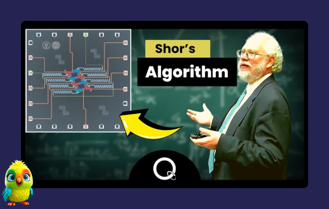
– Example: Shor’s algorithm uses quantum adders for exponential speedup in factorization.
Visualization (Simplified)
Quantum Circuit for 3 + 2:
1. Encode: |11⟩ (3) + |10⟩ (2)
2. Apply quantum gates (CNOT, Toffoli):
|11⟩ + |10⟩ → |101⟩ (5)
3. Measure: 101 (5) with high probability.
Key Takeaways
1. Reversible Gates: Quantum adders avoid information loss (unlike classical NAND gates).
2. Superposition: Can evaluate multiple sums at once (useful for complex problems).
3. Measurement: Output is probabilistic; repeated runs ensure accuracy.
2. Quantum Fundamentals
Wave-Particle Duality
Wave-Particle Duality: The Dual Nature of Quantum Objects
Wave-particle duality is a fundamental concept in quantum mechanics that states every particle (e.g., electrons, photons) exhibits both wave-like and particle-like properties, depending on how it is observed.
1. Historical Background
– Isaac Newton (1700s): Proposed light as particles (“corpuscles”).
– Thomas Young (1801): Demonstrated light’s wave nature via the double-slit experiment (interference patterns).
– Einstein (1905): Explained the photoelectric effect (light as particles, or photons), earning him the Nobel Prize.
– De Broglie (1924): Hypothesized that all matter has wave-like properties (λ = h/p, where λ = wavelength, h = Planck’s constant, p = momentum).
2. Key Experiments
A. Double-Slit Experiment (Wave vs. Particle Behavior)
– Classical Particles (e.g., bullets):
– Shoot bullets → two distinct bands on detector.
– Classical Waves (e.g., water):
– Waves interfere → bright and dark bands (interference pattern).
– Quantum Particles (e.g., electrons or photons):
– Single particles fired one at a time still form an interference pattern (wave-like behavior).
– But if you measure which slit they pass through, they behave like particles (no interference).
Interpretation:
– Quantum objects exist in a superposition of states (passing through both slits) until measured.
– Measurement collapses the wavefunction, forcing a particle-like outcome.
B. Photoelectric Effect (Particle Behavior)
– Light shining on metal ejects electrons only if frequency > threshold (wave theory failed to explain this).
– Einstein showed light delivers energy in discrete packets (photons):
\[
E = hf \quad \text{(Energy of a photon)}
\]
– \( h \) = Planck’s constant (\( 6.626 \times 10^{-34} \, \text{J·s} \)).
– \( f \) = frequency of light.
3. Mathematical Description (De Broglie Wavelength)
All matter has a wavelength associated with it:
\[
\lambda = \frac{h}{p} = \frac{h}{mv}
\]
– \( \lambda \) = wavelength
– \( p \) = momentum (\( p = mv \))
– \( m \) = mass, \( v \) = velocity
Example:
– An electron (\( m = 9.11 \times 10^{-31} \, \text{kg} \)) moving at \( 1 \times 10^6 \, \text{m/s} \):
\[
\lambda = \frac{6.626 \times 10^{-34}}{(9.11 \times 10^{-31})(1 \times 10^6)} \approx 0.73 \, \text{nm}
\]
(Detectable in experiments like electron diffraction.)
4. Interpretations & Implications
A. Complementarity (Bohr)
– A quantum system cannot exhibit wave and particle properties simultaneously in the same experiment.
– The observer’s choice of measurement determines which behavior is observed.
B. Quantum Superposition
– Before measurement, particles exist in a wave-like probability distribution.
– Example: Electron in an atom is not in a fixed position but described by a wavefunction (ψ).
C. Applications
– Electron Microscopes: Use wave nature of electrons for high-resolution imaging.
– Quantum Computing: Relies on superposition and interference of qubits.
5. Thought Experiment: Schrödinger’s Cat
– Illustrates superposition and wave-particle duality.
– A cat in a box is simultaneously alive and dead (wave-like probability) until observed (collapses to one state).
| Aspect | Wave-Like Behavior | Particle-Like Behavior |
|---|---|---|
| Evidence | Double-slit interference | Photoelectric effect |
| Mathematical Rep. | Wavefunction (ψ) | Quantized energy (E = hf) |
| Measurement | Interference patterns | Discrete impacts (e.g., photon hits) |
– Quantum objects exhibit both wave-like and particle-like behavior.
– Described by the Schrödinger equation:
\[
i\hbar \frac{\partial}{\partial t} | \psi(t) \rangle = \hat{H} | \psi(t) \rangle
\]
where \( \hat{H} \) is the Hamiltonian operator.
Conclusion: Wave-particle duality shows that quantum objects are neither purely waves nor particles, but something more complex-a reality governed by probability and observation.
Superposition
Quantum Superposition: The Core of Quantum Weirdness
Superposition is the fundamental principle that a quantum system can exist in multiple states simultaneously until measured. It’s the reason quantum computers can outperform classical ones and why Schrödinger’s cat can be both alive and dead.
1. What is Superposition?
– In classical physics, objects have definite states (e.g., a light switch is on or off).
– In quantum mechanics, particles (e.g., electrons, photons, qubits) can be in a blend of states until observed.
– Mathematically: A quantum state \(|\psi\rangle\) is a linear combination of basis states:
\[
|\psi\rangle = \alpha|0\rangle + \beta|1\rangle
\]
– \(|0\rangle\) and \(|1\rangle\) are basis states (like classical 0 and 1).
– \(\alpha, \beta\) are complex numbers (probability amplitudes), where \(|\alpha|^2 + |\beta|^2 = 1\).
2. Key Experiments Demonstrating Superposition
A. Double-Slit Experiment (Revisited)
– Single particles (electrons/photons) produce an interference pattern even when sent one at a time.
– Interpretation: Each particle passes through both slits in superposition and interferes with itself.
B. Stern-Gerlach Experiment (Spin Superposition)
– Silver atoms shot through a magnetic field split into two paths (spin-up \(|↑\rangle\) and spin-down \(|↓\rangle\)).
– If unmeasured, they exist in superposition:
\[
|\psi\rangle = \frac{1}{\sqrt{2}}|↑\rangle + \frac{1}{\sqrt{2}}|↓\rangle
\]
3. Schrödinger’s Cat (Thought Experiment)
– A cat in a box is:
– Alive if a radioactive atom does not decay.
– Dead if the atom decays (triggering poison release).
– Quantum mechanics says the cat is both alive and dead (superposition) until the box is opened (measurement collapses the state).
4. Superposition in Quantum Computing
Example: Superposition in a Hadamard Gate
– Apply a Hadamard gate to \(|0\rangle\):
\[
H|0\rangle = \frac{|0\rangle + |1\rangle}{\sqrt{2}}
\]
– The qubit is now in a 50/50 superposition of \(|0\rangle\) and \(|1\rangle\).
5. The Measurement Problem
– When you measure a superposition, it collapses to one state (e.g., \(|0\rangle\) or \(|1\rangle\)).
– Probability of outcome:
– \(P(0) = |\alpha|^2\)
– \(P(1) = |\beta|^2\)
Example: Measuring \( \frac{|0\rangle + |1\rangle}{\sqrt{2}} \) gives:
– 50
6. Real-World Applications
1. Quantum Cryptography (QKD)
– Superposition enables unhackable communication (e.g., BB84 protocol).
2. Quantum Algorithms
– Shor’s algorithm (factorization) and Grover’s search leverage superposition for exponential speedup.
3. Quantum Sensors
– Atomic clocks (superposition of energy states) enable ultra-precise timekeeping.
– A quantum system can exist in multiple states at once:
\[
| \psi \rangle = \sum_i c_i | \phi_i \rangle
\]
where \( | \phi_i \rangle \) are basis states.
Entanglement
Quantum Entanglement: Spooky Action at a Distance
Entanglement is a phenomenon where two or more quantum particles become intrinsically linked, such that the state of one instantly influences the other-no matter how far apart they are. Einstein called this “spooky action at a distance,” but it’s a proven feature of quantum mechanics and the backbone of quantum tech.
1. What is Quantum Entanglement?
– Definition: A strong correlation between particles where measuring one determines the state of the other(s), even if separated by light-years.
– Key Property: Entangled particles cannot be described independently – their quantum state is shared.
Example: Bell State (Maximally Entangled Pair)
The simplest entangled system (two qubits):
\[
|\Phi^+\rangle = \frac{|00\rangle + |11\rangle}{\sqrt{2}}
\]
– If Alice measures her qubit as \(|0\rangle\), Bob’s qubit instantly becomes \(|0\rangle\).
– If Alice gets \(|1\rangle\), Bob’s qubit is \(|1\rangle\) – faster than light, but no information is transmitted.
2. How Entanglement Works (Step-by-Step)
Step 1: Create Entanglement
– Method: Use quantum gates (e.g., CNOT + Hadamard) or natural interactions (e.g., photon decay).
– Example:
1. Prepare two qubits: \(|0\rangle_A \otimes |0\rangle_B\).
2. Apply Hadamard to qubit A: \(\frac{|0\rangle + |1\rangle}{\sqrt{2}} \otimes |0\rangle\).
3. Apply CNOT (flips B if A is \(|1\rangle\)): \(\frac{|00\rangle + |11\rangle}{\sqrt{2}}\).
Step 2: Separate the Particles
– Send one qubit to Alice (Earth) and the other to Bob (Mars).
Step 3: Measure One Qubit → Instant Collapse
– Alice measures her qubit:
– If she gets \(|0\rangle\), Bob’s qubit must be \(|0\rangle\).
– If she gets \(|1\rangle\), Bob’s qubit must be \(|1\rangle\).
Key Point: No classical communication happens—the correlation is immediate.
3. Experimental Proof: Bell’s Theorem
– Classical View: Hidden variables predetermine outcomes (local realism).
– Quantum View: Outcomes are truly random until measured (non-locality).
– Alain Aspect (1982): Experiments violated Bell’s inequality, proving entanglement is not explainable by hidden variables.
4. Applications of Entanglement
| Field | Application | How Entanglement Helps |
|---|---|---|
| Computing | Quantum parallelism | Links qubits for exponential speedup (e.g., Shor’s algorithm). |
| Cryptography | Quantum Key Distribution (QKD) | Detects eavesdroppers (any measurement breaks entanglement). |
| Teleportation | Quantum state transfer | Transfers qubit states without physical travel (used in quantum networks). |
| Metrology | Ultra-precise sensors (e.g., LIGO) | Entangled photons improve measurement precision beyond classical limits. |
– Two qubits in an entangled state (e.g., Bell state):
\[
| \Phi^+ \rangle = \frac{1}{\sqrt{2}} (|00\rangle + |11\rangle)
\]
Quantum Measurement
Quantum Measurement: The Collapse of the Wavefunction
Quantum measurement is the process of observing a quantum system, causing its wavefunction to collapse into a definite state. It’s where the weirdness of superposition becomes tangible reality-and it’s the bridge between quantum possibilities and classical outcomes.
1. The Measurement Postulate (Born Rule)
– Before measurement: A quantum system exists in a superposition of states:
\[
|\psi\rangle = \alpha|0\rangle + \beta|1\rangle
\]
– After measurement: The system collapses to either \(|0\rangle\) or \(|1\rangle\) with probabilities:
\[
P(0) = |\alpha|^2, \quad P(1) = |\beta|^2
\]
– Key Point: Measurement destroys superposition and forces a classical outcome.
2. The Measurement Problem
What Happens During Collapse?
– Copenhagen Interpretation: The wavefunction collapses upon observation (no deeper mechanism).
– Many-Worlds Interpretation: All outcomes happen; the universe branches (no collapse).
– Objective Collapse Theories: Wavefunction collapse is a physical process (e.g., gravity-induced).
Schrödinger’s Cat Revisited
– The cat is in superposition (alive + dead) until the box is opened (measurement occurs).
– Paradox: Who/what qualifies as an “observer”? (Consciousness? Detection devices?)
3. Types of Quantum Measurements
A. Projective (Strong) Measurements
– Example: Measuring a qubit in the \(\{|0\rangle, |1\rangle\}\) basis.
– Irreversible: System stays in the collapsed state.
B. Weak Measurements
– Extracts partial info without full collapse (used in quantum sensing).
C. Non-Demolition Measurements
– Measures a property without disturbing others (e.g., photon number in a cavity).
4. Quantum Measurement Devices
| Device | What It Measures | Example |
|---|---|---|
| Stern-Gerlach Apparatus | Electron spin ((↑\rangle, ↓\rangle)) | Splits silver atoms in a magnetic field. |
| Photodetector | Photon presence (0 or 1) | "Clicks" if a photon is absorbed. |
| Interferometer | Phase/position of waves | LIGO (detects gravitational waves). |
5. The Observer Effect vs. Uncertainty Principle
– Observer Effect: Measurement disturbs the system (e.g., photon hitting an electron).
– Uncertainty Principle: Fundamental limit on simultaneous knowledge of pairs (e.g., position/momentum).
Example:
– Measuring an electron’s position changes its momentum unpredictably.
6. Applications of Quantum Measurement
1. Quantum Computing
– Readout of qubits (e.g., superconducting qubits measured via microwave resonators).
2. Quantum Cryptography
– Detecting eavesdroppers (measurement disturbs entangled states).
3. Medical Imaging (MRI)
– Measures nuclear spins in magnetic fields.
7. Controversies & Open Questions
– Does consciousness cause collapse? (Wigner’s Friend thought experiment)
– How fast does collapse happen? (Instantaneous or finite time?)
– Can we avoid collapse? (Quantum Darwinism suggests “objective reality” emerges from decoherence.)
8. Key Equations
– Born Rule: \( P(x) = |\langle x|\psi\rangle|^2 \)
– Heisenberg Uncertainty: \( \Delta x \Delta p \geq \frac{\hbar}{2} \)
Summary
– Measurement forces quantum systems to “choose” a state.
– Collapse is probabilistic (governed by Born’s rule).
– The nature of collapse is still debated (interpretations vary).
Fun Fact: In quantum labs, “measurement” often means amplifying quantum effects to classical scales (e.g., a single photon triggering a macroscopic detector).
– The probability of measuring state \( | \phi_i \rangle \) is:
\[
P(i) = |\langle \phi_i | \psi \rangle|^2
\]
– Post-measurement, the state collapses to \( | \phi_i \rangle \).