Vector Analysis A Comprehensive Treatise from Foundations to Theorems
Prologue: The Language of Physics and Engineering
Part I: The Foundations of Vector Algebra
* Chapter 1: Scalars, Vectors, and Basic Notations
* 1.1: The Fundamental Distinction: Scalars vs. Vectors
* 1.2: Vector Representation and Notation
* 1.3: Position Vectors and Displacement
* Chapter 2: Vector Operations
* 2.1: Vector Addition and Subtraction (Triangle & Parallelogram Laws)
* 2.2: Scalar Multiplication
* 2.3: Magnitude of a Vector
* 2.4: Unit Vectors and Direction Cosines
* Chapter 3: The Dot Product (Scalar Product)
* 3.1: Algebraic and Geometric Definitions
* 3.2: Work Done by a Force
* 3.3: The Angle Between Two Vectors
* 3.4: Orthogonality and Projection
* Chapter 4: The Cross Product (Vector Product)
* 4.1: Algebraic and Geometric Definitions
* 4.2: Torque and Moment of a Force
* 4.3: Area of a Parallelogram and Triangle
* Chapter 5: Triple Products
* 5.1: Scalar Triple Product and the Volume of a Parallelepiped
* 5.2: Vector Triple Product and its Identities
Part II: Vector Calculus - The Heart of Analysis
* Chapter 6: Vector Functions of a Single Variable
* 6.1: Differentiation of Vectors (Velocity, Acceleration)
* 6.2: Integration of Vectors
* Chapter 7: Differential Calculus of Scalar and Vector Fields
* 7.1: The Del (Nabla) Operator, ∇
* 7.2: Gradient of a Scalar Field (∇f)
* 7.3: Directional Derivative (Dᵤf)
* 7.4: Divergence of a Vector Field (∇ ⋅ F)
* 7.5: Curl of a Vector Field (∇ × F)
* 7.6: The Laplacian (∇²f and ∇²F)
* Chapter 8: Curvilinear Coordinates
* 8.1: Cylindrical Coordinates
* 8.2: Spherical Coordinates
* 8.3: Gradient, Divergence, Curl, and Laplacian in Curvilinear Coordinates
* Chapter 9: Integral Theorems of Vector Calculus
* 9.1: The Divergence Theorem (Gauss's Theorem)
* 9.2: Stokes' Theorem
* 9.3: Green's Theorem in the Plane
Part III: Applications and Advanced Concepts
* Chapter 10: Eigenvalues and Eigenvectors in Vector Contexts
* Chapter 11: Vector Potentials and Solenoidal Fields
* Chapter 12: Geometric Applications: Lines and Planes
* 12.1: Equations of Lines and Planes
* 12.2: Angle Between Two Vectors / Planes
* 12.3: Distance Between Points, Lines, and Planes
* Chapter 13: Physical Applications
* 13.1: Bulk Modulus and Stress/Strain Tensors (Introduction)
* 13.2: Fluid Flow and Continuity Equations
* 13.3: Electromagnetism: Maxwell's Equations
Epilogue: The Power of the Vector Language
Appendices
* Appendix A: Tensor Notation (A Brief Overview)
* Appendix B: The Hessian Matrix and Optimization
* Appendix C: Table of Vector Identities
Prologue: The Language of Physics and Engineering
Why do we need vectors? Consider the simple act of navigating. Telling a friend "I walked 5 kilometers" is incomplete. "I walked 5 kilometers *due north*" is complete. The first is a scalar (magnitude only); the second is a vector (magnitude and direction). This distinction is the bedrock of classical physics. Force, velocity, electric field, fluid flow—none of these can be described by a single number. They require a direction. Vector analysis provides the mathematical language to describe, manipulate, and understand these physical quantities. This treatise will guide you from the basic definitions to the profound integral theorems that unite local and global behavior of fields, empowering you to solve complex problems in engineering, physics, and computer science.
*Part I: The Foundations of Vector Algebra
Chapter 1: Scalars, Vectors, and Basic Notations
1.1: The Fundamental Distinction: Scalars vs. Vectors
* Scalar: A quantity that is completely specified by a single real number (its magnitude) and has no direction.
* Examples: Mass (5 kg), Temperature (20 °C), Time (10 s), Volume (3 m³), Density, Energy.
* Notation: Usually denoted by italic letters: \( m, T, t, V \).
* Vector: A quantity that has both magnitude and direction.
* Examples: Displacement (5 m North), Velocity (60 km/h East), Force (10 N downward), Acceleration, Electric Field.
* Notation: Denoted by boldface letters ( v , F ), or with an arrow above (\( \vec{v}, \vec{F} \)). In handwriting, the arrow is essential.
1.2: Vector Representation and Notation
A vector in 3-dimensional space is defined by its three components along the mutually perpendicular x, y, and z axes. The standard unit vectors are:
* \( \hat{\mathbf{i}} \) : Unit vector in the x-direction.
* \( \hat{\mathbf{j}} \) : Unit vector in the y-direction.
* \( \hat{\mathbf{k}} \) : Unit vector in the z-direction.
Any vector \( \vec{A} \) can be written as:
\[\vec{A} = A_x\hat{\mathbf{i}} + A_y\hat{\mathbf{j}} + A_z\hat{\mathbf{k}}\]
where \( A_x, A_y, A_z \) are the scalar components of \( \vec{A} \).
Example 1.2.1: Represent a force of 10 N acting in the x-y plane at a 30° angle to the positive x-axis.
Solution:
The components are:
\[F_x = 10 \cos(30^\circ) = 10 \cdot \frac{\sqrt{3}}{2} = 5\sqrt{3} \, \text{N}\]
\[F_y = 10 \sin(30^\circ) = 10 \cdot \frac{1}{2} = 5 \, \text{N}\]
\[F_z = 0 \, \text{N}\]
Thus, the vector is:
\[\vec{F} = 5\sqrt{3} \, \hat{\mathbf{i}} + 5 \, \hat{\mathbf{j}}\]
1.3: Position Vectors and Displacement
* Position Vector (\( \vec{r} \)): A vector that specifies the location of a point \( P(x, y, z) \) relative to the origin \( O(0, 0, 0) \).
\[\vec{r} = x\hat{\mathbf{i}} + y\hat{\mathbf{j}} + z\hat{\mathbf{k}}\]
* Displacement Vector (\( \Delta \vec{r} \)): The change in position. If an object moves from point \( P_1(x_1, y_1, z_1) \) to \( P_2(x_2, y_2, z_2) \), the displacement is:
\[\Delta \vec{r} = \vec{r}_2 - \vec{r}_1 = (x_2 - x_1)\hat{\mathbf{i}} + (y_2 -y_1)\hat{\mathbf{j}} + (z_2 - z_1)\hat{\mathbf{k}}\]
Crucial Point: Displacement is *not* the same as distance traveled. It is the straight-line vector from the initial to the final position.
Example 1.3.1: A particle moves from \( P(1, 2, 3) \) to \( Q(4, 6, 8) \). Find its displacement vector.
Solution:
\[\vec{r}_P = 1\hat{\mathbf{i}} + 2\hat{\mathbf{j}} + 3\hat{\mathbf{k}}\]
\[\vec{r}_Q = 4\hat{\mathbf{i}} + 6\hat{\mathbf{j}} + 8\hat{\mathbf{k}}\]
\[\Delta \vec{r} = \vec{r}_Q - \vec{r}_P = (4-1)\hat{\mathbf{i}} + (6-2)\hat{\mathbf{j}} + (8-3)\hat{\mathbf{k}} = 3\hat{\mathbf{i}} + 4\hat{\mathbf{j}} + 5\hat{\mathbf{k}}\]
Chapter 2: Vector Operations
2.1: Vector Addition and Subtraction
Vectors add component-wise and obey the commutative and associative laws.
If \( \vec{A} = A_x\hat{\mathbf{i}} + A_y\hat{\mathbf{j}} + A_z\hat{\mathbf{k}} \) and \( \vec{B} = B_x\hat{\mathbf{i}} + B_y\hat{\mathbf{j}} + B_z\hat{\mathbf{k}} \), then:
\[\vec{A} + \vec{B} = (A_x + B_x)\hat{\mathbf{i}} + (A_y + B_y)\hat{\mathbf{j}} + (A_z +B_z)\hat{\mathbf{k}}\]
\[\vec{A} - \vec{B} = (A_x - B_x)\hat{\mathbf{i}} + (A_y - B_y)\hat{\mathbf{j}} + (A_z -B_z)\hat{\mathbf{k}}\]
*Geometrically*, addition is achieved by the Triangle Law (tip-to-tail) or the Parallelogram Law .
Example 2.1.1: Given \( \vec{A} = 2\hat{\mathbf{i}} - \hat{\mathbf{j}} + 3\hat{\mathbf{k}} \) and \( \vec{B} = -\hat{\mathbf{i}} + 4\hat{\mathbf{j}} + 2\hat{\mathbf{k}} \), find \( \vec{A} + \vec{B} \) and \( \vec{A} - \vec{B} \).
Solution:
\[\vec{A} + \vec{B} = (2 + (-1))\hat{\mathbf{i}} + ((-1) + 4)\hat{\mathbf{j}} + (3 + 2)\hat{\mathbf{k}} = 1\hat{\mathbf{i}} + 3\hat{\mathbf{j}} + 5\hat{\mathbf{k}}\]
\[\vec{A} - \vec{B} = (2 - (-1))\hat{\mathbf{i}} + ((-1) - 4)\hat{\mathbf{j}} + (3 -2)\hat{\mathbf{k}} = 3\hat{\mathbf{i}} - 5\hat{\mathbf{j}} + 1\hat{\mathbf{k}}\]
2.2 & 2.3: Scalar Multiplication and Magnitude
* Scalar Multiplication: Multiplying a vector by a scalar \( c \) scales its magnitude by \( |c| \) and reverses its direction if \( c \) is negative.
\[ c\vec{A} = cA_x\hat{\mathbf{i}} + cA_y\hat{\mathbf{j}} + cA_z\hat{\mathbf{k}}\]
* Magnitude (or Norm): The length of the vector, always a non-negative scalar.
\[ |\vec{A}| = A = \sqrt{A_x^2 + A_y^2 + A_z^2} \]
Example 2.3.1: For \( \vec{A} = 3\hat{\mathbf{i}} - 4\hat{\mathbf{j}} + 12\hat{\mathbf{k}} \), find \( |\vec{A}| \) and the vector \( -2\vec{A} \).
Solution:
\[|\vec{A}| = \sqrt{(3)^2 + (-4)^2 + (12)^2} = \sqrt{9 + 16 + 144} = \sqrt{169} = 13\]
\[-2\vec{A} = -2(3\hat{\mathbf{i}} - 4\hat{\mathbf{j}} + 12\hat{\mathbf{k}}) =-6\hat{\mathbf{i}} + 8\hat{\mathbf{j}} - 24\hat{\mathbf{k}}\]
The magnitude of \( -2\vec{A} \) is \( |-2\vec{A}| = \sqrt{(-6)^2 + 8^2 + (-24)^2} = \sqrt{676} = 26 = 2 \times 13 \), as expected.
2.4: Unit Vectors and Direction Cosines
* Unit Vector: A vector with magnitude 1. The unit vector in the direction of \( \vec{A} \) is:
\[\hat{A} = \frac{\vec{A}}{|\vec{A}|}\]
* Direction Cosines: The cosines of the angles \( \alpha, \beta, \gamma \) that the vector makes with the positive x, y, and z axes, respectively.
\[ \cos \alpha = \frac{A_x}{|\vec{A}|}, \quad \cos \beta = \frac{A_y}{|\vec{A}|}, \quad \cos\gamma = \frac{A_z}{|\vec{A}|}\]
Note: \( \cos^2 \alpha + \cos^2 \beta + \cos^2 \gamma = 1 \).
Example 2.4.1: Find the unit vector parallel to \( \vec{B} = \hat{\mathbf{i}} - 2\hat{\mathbf{j}} + 2\hat{\mathbf{k}} \) and its direction cosines.
Solution:
First, find the magnitude:
\[|\vec{B}| = \sqrt{(1)^2 + (-2)^2 + (2)^2} = \sqrt{1 + 4 + 4} = \sqrt{9} = 3\]
The unit vector is:
\[\hat{B} = \frac{\vec{B}}{|\vec{B}|} = \frac{\hat{\mathbf{i}} - 2\hat{\mathbf{j}} + 2\hat{\mathbf{k}}}{3} = \frac{1}{3}\hat{\mathbf{i}} - \frac{2}{3}\hat{\mathbf{j}} + \frac{2}{3}\hat{\mathbf{k}}\]
The direction cosines are:
\[\cos \alpha = \frac{1}{3}, \quad \cos \beta = -\frac{2}{3}, \quad \cos \gamma = \frac{2}{3}\]
Chapter 3: The Dot Product (Scalar Product)
3.1: Algebraic and Geometric Definitions
The dot product of two vectors \( \vec{A} \) and \( \vec{B} \) results in a scalar .
* Algebraic Definition:
\[\vec{A} \cdot \vec{B} = A_xB_x + A_yB_y + A_zB_z \]
* Geometric Definition:
\[\vec{A} \cdot \vec{B} = |\vec{A}|\, |\vec{B}| \cos \theta\]
where \( \theta \) is the angle between the two vectors (\( 0 \leq \theta \leq \pi \)).
These definitions are equivalent. The geometric definition is often used to find the angle between two vectors.
3.2: Work Done by a Force
This is the quintessential physical application of the dot product. Work is defined as the product of the displacement and the component of the force in the direction of displacement.
\[W = \vec{F} \cdot \Delta \vec{r} = |\vec{F}|\, |\Delta \vec{r}| \cos \theta\]
If the force is perpendicular to the displacement, no work is done (\( \cos 90^\circ = 0 \)).
Example 3.2.1: A force \( \vec{F} = 3\hat{\mathbf{i}} + 4\hat{\mathbf{j}} \, \text{N} \) acts on an object, displacing it by \( \Delta \vec{r} = 5\hat{\mathbf{i}} \, \text{m} \). Calculate the work done.
Solution:
Using the algebraic definition:
\[W = \vec{F} \cdot \Delta \vec{r} = (3)(5) + (4)(0) + (0)(0) = 15 \, \text{Joules}\]
Using the geometric definition: \( |\vec{F}| = 5 \, \text{N} \), \( |\Delta \vec{r}| = 5 \, \text{m} \), \( \theta \) is the angle between \( 3\hat{\mathbf{i}}+4\hat{\mathbf{j}} \) and \( 5\hat{\mathbf{i}} \), so \( \cos \theta = 3/5 \). Thus, \( W = (5)(5)(3/5) = 15 \, \text{J} \).
3.3 & 3.4: Angle Between Vectors and Orthogonality
From the geometric definition, we can solve for the angle:
\[\theta = \cos^{-1} \left( \frac{\vec{A} \cdot \vec{B}}{|\vec{A}|\, |\vec{B}|} \right)\]
Two vectors are orthogonal (perpendicular) if and only if their dot product is zero.
\[\vec{A} \perp \vec{B} \iff \vec{A} \cdot \vec{B} = 0\]
Example 3.4.1: Show that \( \vec{A} = 2\hat{\mathbf{i}} + 3\hat{\mathbf{j}} - \hat{\mathbf{k}} \) and \( \vec{B} = \hat{\mathbf{i}} - 2\hat{\mathbf{j}} - 4\hat{\mathbf{k}} \) are orthogonal.
Solution:
Compute the dot product:
\[\vec{A} \cdot \vec{B} = (2)(1) + (3)(-2) + (-1)(-4) = 2 - 6 + 4 = 0\]
Since the dot product is zero, the vectors are orthogonal.
*(This structure continues for all chapters listed in the Table of Contents. Each chapter would contain:*
- *Conceptual explanations with clear, professor-level insights.*
- *Precise mathematical definitions and formulas.*
- *Worked examples with detailed solutions, illustrating both computation and conceptual understanding.*
- *Connections to physics and engineering where appropriate.*
- *Diagrams for geometric interpretation (e.g., for cross product, gradient, etc.).)*
A Glimpse into Later Chapters:
Chapter 7.5: Curl (Kerl) of a Vector Field
The curl, denoted \( \nabla \times \vec{F} \), measures the infinitesimal circulation or "rotationality" of a vector field at a point. Imagine placing a tiny paddlewheel in a fluid flow; the curl tells you if and how fast it will spin.
* Definition in Cartesian Coordinates:
\[\nabla \times \vec{F} = \begin{vmatrix} \hat{\mathbf{i}} & \hat{\mathbf{j}} & \hat{\mathbf{k}} \\ \frac{\partial}{\partial x} & \frac{\partial}{\partial y} & \frac{\partial}{\partial z} \\ F_x & F_y & F_z \end{vmatrix} = \left( \frac{\partial F_z}{\partial y} - \frac{\partial F_y}{\partial z} \right) \hat{\mathbf{i}} + \left( \frac{\partial F_x}{\partial z} - \frac{\partial F_z}{\partial x} \right) \hat{\mathbf{j}} + \left( \frac{\partial F_y}{\partial x} - \frac{\partial F_x}{\partial y} \right) \hat{\mathbf{k}}\]
* Physical Meaning:
* \( \nabla \times \vec{F} = \vec{0} \): The field is irrotational (e.g., electrostatic field).
* \( \nabla \times \vec{F} \neq \vec{0} \): The field has rotation (e.g., the velocity field of a vortex).
Example 7.5.1: Calculate the curl of \( \vec{F} = -y\hat{\mathbf{i}} + x\hat{\mathbf{j}} \).
Solution:
\[\nabla \times \vec{F} = \begin{vmatrix} \hat{\mathbf{i}} & \hat{\mathbf{j}} & \hat{\mathbf{k}} \\ \frac{\partial}{\partial x} & \frac{\partial}{\partial y} & \frac{\partial}{\partial z} \\ -y & x & 0\end{vmatrix}\] \[= \hat{\mathbf{i}} \left( \frac{\partial (0)}{\partial y} - \frac{\partial (x)}{\partial z} \right) - \hat{\mathbf{j}} \left( \frac{\partial (0)}{\partial x} - \frac{\partial (-y)}{\partial z} \right) + \hat{\mathbf{k}} \left( \frac{\partial (x)}{\partial x} - \frac{\partial (-y)}{\partial y} \right)\] \[= \hat{\mathbf{i}}(0 - 0) - \hat{\mathbf{j}}(0 - 0) + \hat{\mathbf{k}}(1 - (-1)) = 0\hat{\mathbf{i}} - 0\hat{\mathbf{j}} + 2\hat{\mathbf{k}} = 2\hat{\mathbf{k}}\]
This confirms the field has a constant rotation about the z-axis.
7.6: The Laplacian Operator (∇²)
The Laplacian is a fundamental differential operator of second order, appearing ubiquitously in physics: heat equation, wave equation, Laplace's equation, quantum mechanics, and fluid dynamics.
Definition: The Laplacian of a scalar field \( f \) is the divergence of the gradient of \( f \).
\[ \nabla^2 f = \nabla \cdot (\nabla f) = \text{div}(\text{grad } f) \]
In Cartesian Coordinates:
\[ \nabla^2 f = \frac{\partial^2 f}{\partial x^2} + \frac{\partial^2 f}{\partial y^2} + \frac{\partial^2 f}{\partial z^2} \]
Physical Interpretation: The Laplacian \( \nabla^2 f \) at a point measures the difference between the average value of \( f \) around a point and its value at the point itself. It quantifies the "smoothness" or "diffusion" of a field.
* \( \nabla^2 f > 0 \): The point is at a lower potential than its surroundings (a valley).
* \( \nabla^2 f < 0 \): The point is at a higher potential than its surroundings (a peak).
* \( \nabla^2 f = 0 \): The function is harmonic (Laplace's equation), meaning its value at any point is the average of its values in the neighborhood.
Example 7.6.1: Compute the Laplacian of \( f(x, y, z) = 3x^2 + \sin(y) - e^z \).
Solution:
Compute the second partial derivatives:
\[ \frac{\partial f}{\partial x} = 6x, \quad \frac{\partial^2 f}{\partial x^2} = 6 \]
\[ \frac{\partial f}{\partial y} = \cos(y), \quad \frac{\partial^2 f}{\partial y^2} = -\sin(y) \]
\[ \frac{\partial f}{\partial z} = -e^z, \quad \frac{\partial^2 f}{\partial z^2} = -e^z \]
Summing them gives the Laplacian:
\[ \nabla^2 f = 6 + (-\sin(y)) + (-e^z) = 6 - \sin(y) - e^z \]
Vector Laplacian: The Laplacian can also be applied to a vector field \( \vec{F} \). It is defined component-wise:
\[ \nabla^2 \vec{F} = (\nabla^2 F_x) \hat{\mathbf{i}} + (\nabla^2 F_y) \hat{\mathbf{j}} + (\nabla^2 F_z) \hat{\mathbf{k}} \]
This identity is often more useful for computation:
\[ \nabla^2 \vec{F} = \nabla(\nabla \cdot \vec{F}) - \nabla \times (\nabla \times \vec{F}) \]
Chapter 8: Curvilinear Coordinates
Many physical systems possess inherent symmetry (cylindrical, spherical) that makes Cartesian coordinates cumbersome. Curvilinear coordinates are more natural and powerful for these problems.
8.1: Cylindrical Coordinates (ρ, φ, z)
Cylindrical coordinates are ideal for problems with axial symmetry (e.g., pipes, wires).
* Coordinates:
* \( \rho \): Radial distance from the z-axis (\( \rho \geq 0 \))
* \( \phi \): Azimuthal angle from the positive x-axis (\( 0 \leq \phi < 2\pi \))
* \( z \): Vertical height (same as Cartesian)
* Relation to Cartesian:
\[ x = \rho \cos\phi, \quad y = \rho \sin\phi, \quad z = z \]
\[ \rho = \sqrt{x^2 + y^2}, \quad \phi = \tan^{-1}(y/x), \quad z = z \]
* Unit Vectors: The unit vectors are orthogonal and point in the direction of increasing coordinate.
* \( \hat{\mathbf{\rho}} \): Points radially outward from the z-axis.
* \( \hat{\mathbf{\phi}} \): Points in the direction of increasing \( \phi \) (tangent to circle).
* \( \hat{\mathbf{z}} \): Points in the positive z-direction.
Crucial Difference: In Cartesian, \( \hat{\mathbf{i}}, \hat{\mathbf{j}}, \hat{\mathbf{k}} \) are constant. In cylindrical, \( \hat{\mathbf{\rho}} \) and \( \hat{\mathbf{\phi}} \) change direction depending on the point in space.
8.2: Spherical Coordinates (r, θ, φ)
Spherical coordinates are ideal for problems with spherical symmetry (e.g., atoms, gravitational fields, sound waves).
* Coordinates:
* \( r \): Radial distance from the origin (\( r \geq 0 \))
* \( \theta \): Polar (zenith) angle from the positive z-axis (\( 0 \leq \theta \leq \pi \))
* \( \phi \): Azimuthal angle from the positive x-axis (\( 0 \leq \phi < 2\pi \)) (Same as cylindrical)
* Relation to Cartesian:
\[ x = r \sin\theta \cos\phi, \quad y = r \sin\theta \sin\phi, \quad z = r \cos\theta \]
\[ r = \sqrt{x^2 + y^2 + z^2}, \quad \theta = \cos^{-1}\left(\frac{z}{r}\right), \quad \phi = \tan^{-1}(y/x) \]
* Unit Vectors:
* \( \hat{\mathbf{r}} \): Points radially outward from the origin.
* \( \hat{\mathbf{\theta}} \): Points "south" along a line of longitude.
* \( \hat{\mathbf{\phi}} \): Points "east" along a line of latitude.
8.3: Vector Operators in Curvilinear Coordinates
The forms of gradient, divergence, curl, and Laplacian are more complex in curvilinear coordinates due to the non-constant unit vectors. They are derived using the metric coefficients of the coordinate systems.
Cylindrical Coordinates (ρ, φ, z):
* Gradient: \( \nabla f = \frac{\partial f}{\partial \rho} \hat{\boldsymbol{\rho}} + \frac{1}{\rho} \frac{\partial f}{\partial \phi} \hat{\boldsymbol{\phi}} + \frac{\partial f}{\partial z} \hat{\mathbf{z}} \)
* Divergence: \( \nabla \cdot \vec{F} = \frac{1}{\rho} \frac{\partial (\rho F_\rho)}{\partial \rho} + \frac{1}{\rho} \frac{\partial F_\phi}{\partial \phi} + \frac{\partial F_z}{\partial z} \)
* Curl:
\[ \nabla \times \vec{F} = \frac{1}{\rho} \begin{vmatrix} \hat{\boldsymbol{\rho}} & \rho\hat{\boldsymbol{\phi}} & \hat{\mathbf{z}} \\ \frac{\partial}{\partial \rho} & \frac{\partial}{\partial \phi} & \frac{\partial}{\partial z} \\ F_\rho & \rho F_\phi & F_z \end{vmatrix} \]
* Laplacian: \( \nabla^2 f = \frac{1}{\rho} \frac{\partial}{\partial \rho} \left( \rho \frac{\partial f}{\partial \rho} \right) + \frac{1}{\rho^2} \frac{\partial^2 f}{\partial \phi^2} + \frac{\partial^2 f}{\partial z^2} \)
Spherical Coordinates (r, θ, φ):
* Gradient: \( \nabla f = \frac{\partial f}{\partial r} \hat{\mathbf{r}} + \frac{1}{r} \frac{\partial f}{\partial \theta} \hat{\boldsymbol{\theta}} + \frac{1}{r \sin\theta} \frac{\partial f}{\partial \phi} \hat{\boldsymbol{\phi}} \)
* Divergence: \( \nabla \cdot \vec{F} = \frac{1}{r^2} \frac{\partial (r^2 F_r)}{\partial r} + \frac{1}{r \sin\theta} \frac{\partial (\sin\theta F_\theta)}{\partial \theta} + \frac{1}{r \sin\theta} \frac{\partial F_\phi}{\partial \phi} \)
* Curl:
\[ \nabla \times \vec{F} = \frac{1}{r^2 \sin\theta} \begin{vmatrix} \hat{\mathbf{r}} & r\hat{\boldsymbol{\theta}} & r\sin\theta\hat{\boldsymbol{\phi}} \\ \frac{\partial}{\partial r} & \frac{\partial}{\partial \theta} & \frac{\partial}{\partial \phi} \\ F_r & r F_\theta & r\sin\theta F_\phi \end{vmatrix} \]
* Laplacian: \( \nabla^2 f = \frac{1}{r^2} \frac{\partial}{\partial r} \left( r^2 \frac{\partial f}{\partial r} \right) + \frac{1}{r^2 \sin\theta} \frac{\partial}{\partial \theta} \left( \sin\theta \frac{\partial f}{\partial \theta} \right) + \frac{1}{r^2 \sin^2\theta} \frac{\partial^2 f}{\partial \phi^2} \)
Example 8.3.1: Find the divergence of \( \vec{F} = \rho^2 \hat{\boldsymbol{\rho}} + z \sin(\phi) \hat{\boldsymbol{\phi}} \) in cylindrical coordinates.
Solution:
Here, \( F_\rho = \rho^2 \), \( F_\phi = z \sin\phi \), \( F_z = 0 \).
Using the formula for divergence in cylindrical coordinates:
\[\nabla \cdot \vec{F} = \frac{1}{\rho} \frac{\partial (\rho F_\rho)}{\partial\rho} + \frac{1}{\rho} \frac{\partial F_\phi}{\partial \phi} +\frac{\partial F_z}{\partial z}
\]
\[= \frac{1}{\rho} \frac{\partial (\rho \cdot \rho^2)}{\partial \rho} +\frac{1{\rho} \frac{\partial (z \sin\phi)}{\partial \phi} + \frac{\partial (0){\partial z}\]
\[= \frac{1}{\rho} \frac{\partial (\rho^3)}{\partial \rho} + \frac{1}{\rho} (z\cos\phi) + 0\]
\[= \frac{1}{\rho} (3\rho^2) + \frac{z \cos\phi}{\rho} = 3\rho + \frac{z\cos\phi}{\rho}\]
Chapter 9: Integral Theorems of Vector Calculus
These theorems are the crown jewels of vector calculus. They provide a profound connection between the behavior of a field inside a region (a volume integral) and its behavior on the boundary of that region (a surface or line integral).
9.1: The Divergence Theorem (Gauss's Theorem)
Theorem: The total "outflow" of a vector field through a closed surface is equal to the total "production" of the field inside the volume enclosed by the surface.
\[\iint_{\partial V} \vec{F} \cdot d\vec{S} = \iiint_V (\nabla \cdot \vec{F}) \, dV\]
* \( S \): A closed, piecewise-smooth surface (e.g., a sphere, a cube).
* \( V \): The volume enclosed by \( S \).
* \( d\vec{S} \): The vector area element, pointing outward (normal to the surface).
Physical Interpretation: If \( \vec{F} \) is the velocity field of a fluid, the LHS is the total flux (flow rate) out of the surface. The RHS is the integral of the source density inside the volume. The theorem says they are equal.
Example 9.1.1: Verify the Divergence Theorem for \( \vec{F} = x\hat{\mathbf{i}} + y\hat{\mathbf{j}} + z\hat{\mathbf{k}} \) over the sphere of radius \( R \), centered at the origin.
Solution:
Volume Integral (RHS):
First, compute the divergence: \( \nabla \cdot \vec{F} = \frac{\partial x}{\partial x} + \frac{\partial y}{\partial y} + \frac{\partial z}{\partial z} = 3 \).
The volume integral is:
\[\iiint_V (\nabla \cdot \vec{F}) \, dV = \iiint_V 3 \, dV = 3 \times(\text{Volume of sphere}) = 3 \cdot \frac{4}{3}\pi R^3 = 4\pi R^3\]
Surface Integral (LHS):
The outward normal to a sphere is \( \hat{\mathbf{r}} \). On the surface, \( \vec{F} = x\hat{\mathbf{i}} + y\hat{\mathbf{j}} + z\hat{\mathbf{k}} = R \hat{\mathbf{r}} \).
Thus, \( \vec{F} \cdot d\vec{S} = (R \hat{\mathbf{r}}) \cdot (\hat{\mathbf{r}} \, dS) = R \, dS \).
The surface integral is:
\[\iint_{\partial V} \vec{F} \cdot d\vec{S} = \iint_{\partial V} R \, dS = R \times (\text{Surface Area of sphere}) = R \cdot 4\pi R^2 = 4\pi R^3\]
Both sides equal \( 4\pi R^3 \), verifying the theorem.
9.2: Stokes' Theorem
Theorem: The circulation of a vector field around a closed loop is equal to the total flux of its curl through any surface bounded by the loop.
\[ \oint_C \vec{F} \cdot d\vec{r} = \iint_S (\nabla \times \vec{F}) \cdot d\vec{S} \]
* \( C \): A simple, closed, piecewise-smooth curve.
* \( S \): Any piecewise-smooth surface bounded by \( C \).
* \( d\vec{r} \): The differential displacement vector along \( C \).
* The direction of \( d\vec{S} \) is given by the right-hand rule relative to the traversal of \( C \).
Physical Interpretation: If \( \vec{F} \) is a force field, the LHS is the work done around a closed path. Stokes' Theorem says this is equal to the flux of the "vorticity" or "rotationality" (\( \nabla \times \vec{F} \)) through the surface.
Example 9.2.1: Verify Stokes' Theorem for \( \vec{F} = -y\hat{\mathbf{i}} + x\hat{\mathbf{j}} \) and the surface \( S \) being the hemisphere \( z = \sqrt{1 - x^2 - y^2} \), with the boundary curve \( C \) being the circle \( x^2 + y^2 = 1 \) in the plane \( z=0 \).
Solution:
Line Integral (LHS):
Parameterize the curve \( C \): \( \vec{r}(t) = \cos t \, \hat{\mathbf{i}} + \sin t \, \hat{\mathbf{j}} + 0\hat{\mathbf{k}}, \quad 0 \leq t \leq 2\pi \).
Then \( d\vec{r}/dt = -\sin t \, \hat{\mathbf{i}} + \cos t \, \hat{\mathbf{j}} \).
On \( C \), \( \vec{F} = -y\hat{\mathbf{i}} + x\hat{\mathbf{j}} = -\sin t \, \hat{\mathbf{i}} + \cos t \, \hat{\mathbf{j}} \).
\[\vec{F} \cdot \frac{d\vec{r}}{dt} = (-\sin t)(-\sin t) + (\cos t)(\cos t) =\sin^2 t + \cos^2 t = 1\]
\[\oint_C \vec{F} \cdot d\vec{r} = \int_0^{2\pi} \left( \vec{F} \cdot\frac{d\vec{r}}{dt} \right) dt = \int_0^{2\pi} 1 \, dt = 2\pi\]
Surface Integral (RHS):
We already computed the curl of this field in a previous example: \( \nabla \times \vec{F} = 2\hat{\mathbf{k}} \).
We need \( \iint_S (\nabla \times \vec{F}) \cdot d\vec{S} \). For the hemisphere, the outward normal is \( \hat{\mathbf{r}} \), but we must be consistent with the right-hand rule from \( C \). For the given traversal (counterclockwise when viewed from above), the correct normal for Stokes' theorem is *upward*, i.e., it has a positive \( z \)-component. The standard unit normal for the hemisphere \( z = \sqrt{1-x^2-y^2} \) is \( \hat{\mathbf{n}} = x\hat{\mathbf{i}} + y\hat{\mathbf{j}} + z\hat{\mathbf{k}} \), which is outward and upward.
The vector surface element is \( d\vec{S} = \hat{\mathbf{n}} \, dS \).
\[(\nabla \times \vec{F}) \cdot d\vec{S} = (2\hat{\mathbf{k}}) \cdot(x\hat{\mathbf{i}} + y\hat{\mathbf{j}} + z\hat{\mathbf{k}}) \, dS = 2z\, dS\]
It's easier to project onto the \( xy \)-plane. For a surface \( z = g(x, y) \), \( dS = \sqrt{1 + (g_x)^2 + (g_y)^2} \, dx\, dy \). Here, \( g(x, y) = \sqrt{1-x^2-y^2} \), so \( dS = \frac{1}{\sqrt{1-x^2-y^2}} \, dx\, dy \).
Also, \( z = \sqrt{1-x^2-y^2} \) on the surface.
Thus, \( (\nabla \times \vec{F}) \cdot d\vec{S} = 2z \, dS = 2\sqrt{1-x^2-y^2} \cdot \frac{1}{\sqrt{1-x^2-y^2}} \, dx\, dy = 2 \, dx\, dy \).
The surface \( S \) projects onto the disk \( R: x^2 + y^2 \leq 1 \) in the \( xy \)-plane.
\[\iint_S (\nabla \times \vec{F}) \cdot d\vec{S} = \iint_R 2 \, dx\, dy = 2\times (\text{Area of disk}) = 2 \cdot \pi (1)^2 = 2\pi\]
Both sides equal \( 2\pi \), verifying the theorem.
9.3: Green's Theorem in the Plane
Green's Theorem is a special case of Stokes' Theorem, confined to a flat plane (e.g., the \( xy \)-plane).
Theorem: Let \( C \) be a positively oriented, piecewise-smooth, simple closed curve in the plane, and let \( D \) be the region bounded by \( C \). If \( P(x, y) \) and \( Q(x, y) \) have continuous partial derivatives on an open region that contains \( D \), then
\[\oint_C (P \, dx + Q \, dy) = \iint_D \left( \frac{\partial Q}{\partial x} -\frac{\partial P}{\partial y} \right) dA\]
Connection to Stokes' Theorem: If we take \( \vec{F} = P\hat{\mathbf{i}} + Q\hat{\mathbf{j}} + 0\hat{\mathbf{k}} \) and a flat surface \( D \) in the \( xy \)-plane, then \( (\nabla \times \vec{F}) \cdot \hat{\mathbf{k}} = \frac{\partial Q}{\partial x} - \frac{\partial P}{\partial y} \). Stokes' Theorem then reduces directly to Green's Theorem.
Example 9.3.1: Use Green's Theorem to evaluate \( \oint_C (y^2 dx + x^2 dy) \), where \( C \) is the triangle with vertices (0,0), (1,0), and (1,1), oriented counterclockwise.
Solution:
Here, \( P = y^2 \), \( Q = x^2 \).
Compute \( \frac{\partial Q}{\partial x} - \frac{\partial P}{\partial y} = 2x - 2y \).
The region \( D \) is a triangle. We can describe it as: \( 0 \leq x \leq 1 \), \( 0 \leq y \leq x \).
Apply Green's Theorem:
\[\oint_C (y^2 dx + x^2 dy) = \iint_D (2x - 2y) \, dA = \int_{x=0}^{1}\int_{y=0}^{x} (2x - 2y) \, dy \, dx\]
First, integrate with respect to \( y \):
\[\int_{y=0}^{x} (2x - 2y) \, dy = \left[ 2xy - y^2 \right]_{0}^{x} = (2x^2 -x^2) - 0 = x^2\]
Now, integrate with respect to \( x \):
\[\int_{x=0}^{1} x^2 \, dx = \left[ \frac{x^3}{3} \right]_{0}^{1} = \frac{1}{3}\]
Thus, the value of the line integral is \( \frac{1}{3} \).
*(This structure and depth would continue for the remaining chapters in Part III, covering Eigenvalues, Vector Potentials, Geometric Applications, and Physical Applications, complete with definitions, theorems, derivations, and worked examples.)*
Epilogue: The Power of the Vector Language
The journey from defining a simple vector to wielding the profound power of the Divergence and Stokes' Theorems reveals a beautiful unification in mathematics and physics. The language of vectors allows us to express physical laws in a way that is independent of any coordinate system, revealing their intrinsic geometric nature. Maxwell's equations of electromagnetism, the Navier-Stokes equations of fluid dynamics, and the principles of continuum mechanics are all most elegantly expressed in this language. Mastering vector analysis is not merely an academic exercise; it is the acquisition of the fundamental toolkit for describing and understanding the physical world.