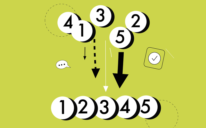
Linear Sorting Algorithms A Theoretical and Practical Deep Dive
Abstract: While comparison-based sorting algorithms like Quicksort and Mergesort form the bedrock of general-purpose sorting, achieving a theoretical lower bound of Ω(n log n) , a separate class of algorithms exists that can shatter this barrier under specific conditions. These are the Linear Sorting Algorithms , which operate in O(n) time by exploiting the inherent structure and properties of the data itself. This comprehensive treatise delves into the three principal linear sorting algorithms-Counting Sort, Radix Sort, and Bucket Sort-exploring their foundational mechanics, rigorous complexity analyses, ideal and pathological use cases, and their profound applications in real-world systems from database management to high-performance computing.
Table of Contents
- Introduction: The Paradigm Shift Beyond Comparison
* 1.1. The Comparison-Based Sorting Lower Bound
* 1.2. The Linear Sorting Hypothesis: Trading Information for Speed
* 1.3. A Taxonomy of Linear Sorts
- Counting Sort: The Art of Tallying and Reconstruction
* 2.1. Foundational Principle: The Frequency Distribution
* 2.2. The Algorithm: A Step-by-Step Conceptual Walkthrough
* 2.3. Complexity Analysis: The `n` and the `k`
* 2.4. The Crucial Property of Stability
* 2.5. Ideal Use Cases and Real-World Applications
* 2.6. Limitations and Pathological Cases
- Radix Sort: The Hierarchical Digit-by-Digit Approach
* 3.1. Foundational Principle: Positional Notation and Significance
* 3.2. LSD vs. MSD: Two Philosophical Approaches
* 3.3. The Role of a Stable Subroutine Algorithm
* 3.4. Complexity Analysis: The `n` and the `d`
* 3.5. Ideal Use Cases and Real-World Applications
* 3.6. Limitations and Pathological Cases
- Bucket Sort: The Divide, Conquer, and Combine Strategy
* 4.1. Foundational Principle: Probabilistic Uniform Distribution
* 4.2. The Algorithm: Scattering, Sorting, and Gathering
* 4.3. The Interplay with Insertion Sort
* 4.4. Complexity Analysis: The Expectation vs. The Worst-Case
* 4.5. Ideal Use Cases and Real-World Applications
* 4.6. Limitations and Pathological Cases
- Comparative Synthesis: Choosing the Right Tool
* 5.1. A Decision Matrix for Algorithm Selection
* 5.2. Hybrid Approaches in Modern Systems
- *Conclusion: The Informed Art of Linear Sorting
- Introduction: The Paradigm Shift Beyond Comparison
1.1. The Comparison-Based Sorting Lower Bound
In the realm of comparison-based sorting, algorithms operate by repeatedly asking one fundamental question: "Is element A greater than element B?" The entire sorting process is a sequence of such pairwise comparisons. A fundamental result in computer science, derived from information theory and decision trees, is that any comparison-based sorting algorithm must make at least Ω(n log n) comparisons in the worst case to correctly sort a list of `n` elements. This is the ceiling for algorithms like Quicksort, Mergesort, and Heapsort. They are general-purpose and make no assumptions about the data they sort.
1.2. The Linear Sorting Hypothesis: Trading Information for Speed
Linear sorting algorithms bypass the `n log n` barrier not by being "smarter" in their comparisons, but by refusing to compare altogether . They achieve this feat by leveraging pre-existing knowledge about the data. This knowledge acts as a "cheat sheet," allowing the algorithm to place elements directly into their correct sorted positions.
The key trade-off is Information for Speed . The required information is typically one of the following:
* Bounded Range (Counting Sort): The data are integers within a known, limited range `k`.
* Compositional Structure (Radix Sort): The data can be broken down into digits, characters, or other components.
* Statistical Distribution (Bucket Sort): The data is uniformly distributed across a known interval.
By exploiting this auxiliary information, linear sorts achieve a time complexity of O(n) , a significant asymptotic improvement over O(n log n) for large `n`.
1.3. A Taxonomy of Linear Sorts
This article focuses on the three canonical linear sorting algorithms:
- *Counting Sort: Operates by counting the frequency of distinct keys.
- *Radix Sort: Sorts data digit by digit, from least significant to most significant (LSD) or vice versa (MSD).
- *Bucket Sort: Distributes elements into several buckets and sorts the buckets individually.
- Counting Sort: The Art of Tallying and Reconstruction
2.1. Foundational Principle: The Frequency Distribution
Counting Sort is built upon a simple, powerful idea: if you know the exact frequency of every distinct value in your dataset, you can reconstruct the sorted list directly. It does not sort by moving elements around through swaps; instead, it deduces the final sorted order.
Real-Life Analogy: The Conference Badge Desk
Imagine you are organizing a conference for 500 attendees. The attendees are assigned a badge based on their company: "A", "B", or "C". As people arrive chaotically, you don't try to sort them physically by shoving them around. Instead, you set up three boxes labeled A, B, and C. As each person arrives, you check their company and drop a pre-made badge into the corresponding box. At the end, you simply output all badges from box A, then all from box B, then all from box C. You have "sorted" 500 people by only performing 500 "lookup" operations.
2.2. The Algorithm: A Step-by-Step Conceptual Walkthrough
Let's sort the array: `[4, 2, 2, 8, 3, 3, 1]`
- *Determine the Range: Find the minimum and maximum value. Here, min=1, max=8. The range `k` = 8 - 1 + 1 = 8.
- *Create the Count Array: Instantiate an array `count` of size `k` (indexed 1 to 8), initialized to zero. This array will represent the frequency of each number.
* `count[1..8] = [0, 0, 0, 0, 0, 0, 0, 0]`
- *The Counting Pass (Tallying): Traverse the input array. For each element, increment the corresponding index in the count array.
* See `4` -> increment `count[4]`. `count` becomes `[0, 0, 0, 1, 0, 0, 0, 0]`
* See `2` -> increment `count[2]`. `count` becomes `[0, 1, 0, 1, 0, 0, 0, 0]`
* ... continue ...
* Final `count` array: `[1, 2, 2, 1, 0, 0, 0, 1]` (Meaning: one '1', two '2's, two '3's, one '4', one '8').
- *Transform Count to Cumulative Count: Modify the count array so that each entry stores the sum of all previous counts. This new value represents the *last* position (1-based) for that element in the sorted array.
* Cumulative `count`: `[1, 3, 5, 6, 6, 6, 6, 7]` (Meaning: the number '1' ends at position 1, '2' ends at position 3, '3' ends at position 5, etc.)
- *The Reconstruction Pass (Building the Output): Create an output array of size `n`. Traverse the *original* array *backwards* (this is crucial for stability).
* Take the last element of the input: `1`. Look up `count[1]`, which is `1`. So, place `1` at position 1 in the output. Decrement `count[1]` to 0.
* Next element: `3`. `count[3]` is `5`. Place `3` at position 5. Decrement `count[3]` to 4.
* ... continue until the first element is processed ...
* The output array is now the sorted list.
2.3. Complexity Analysis: The `n` and the `k`
* Time Complexity: O(n + k). The algorithm makes two passes over the input array (O(n)) and one pass over the count array of size `k` (O(k)).
* Space Complexity: O(k). The primary extra space is the count array of size `k`. The output array is generally not counted as extra space, but if it is, the complexity becomes O(n + k).
The `k` Factor: Counting Sort is linear only if `k = O(n)`. If `k` is very large (e.g., sorting a list of a few numbers where one value is 1,000,000,000), the algorithm becomes impractical, as it requires initializing a gigantic array, wasting both time and memory.
2.4. The Crucial Property of Stability
The step of iterating through the original array *backwards* during reconstruction is what makes Counting Sort stable . Stability means that items with equal value appear in the output in the same order as they appeared in the input. This is critically important when sorting by multiple keys (e.g., sort by last name, then by first name).
2.5. Ideal Use Cases and Real-World Applications
* Sorting Small-Range Integers: Sorting exam scores (0-100), employee ages (18-65), or pixel values (0-255).
* As a Subroutine for Radix Sort: Radix Sort uses Counting Sort as its stable sorting subroutine for each digit.
* Histogram Generation: The counting phase is essentially building a histogram, which is directly useful in image processing.
* Database Query Processing: For aggregations and GROUP BY operations on integer keys with limited distinct values.
2.6. Limitations and Pathological Cases
* Large Value Range (`k >> n`): It is inefficient and often impossible to sort an array `[1, 1000000, 500]` using Counting Sort due to the massive `k`.
* Non-Integer Data: It cannot directly sort strings or floating-point numbers without significant modification (e.g., converting them to integer keys via hashing, which can be complex).
- Radix Sort: The Hierarchical Digit-by-Digit Approach
3.1. Foundational Principle: Positional Notation and Significance
Radix Sort is a clever algorithm that sorts data by processing it in multiple passes, each pass sorting based on a single digit, character, or piece of the key. The core insight is that it's easier to sort `n` elements by a single digit (which has a small, fixed range) than to sort them by their entire value.
Real-Life Analogy: The Librarian's Sorting Strategy
A librarian needs to sort a pile of books by their call numbers (e.g., DDC numbers like 523.1, 004.5, 123.9). A smart strategy is to first sort all books only by the digit in the *ones* place (the last digit). She creates ten piles (0-9) based on this last digit. Then, she collects the piles in order (pile 0, then pile 1, ... pile 9). Now, she sorts this new, partially ordered stack *again*, but this time by the *tenths* place. She repeats this for the hundreds place. After three passes, the books are perfectly sorted. Each pass was a simple task of binning into 10 categories.
3.2. LSD vs. MSD: Two Philosophical Approaches
* Least Significant Digit (LSD) Radix Sort: Starts sorting from the rightmost digit to the leftmost. It is the more common and simpler-to-implement variant. It requires a stable sorting subroutine for the digit-wise sort. The entire list becomes sorted only after the final (most significant digit) pass.
* Most Significant Digit (MSD) Radix Sort: Starts from the leftmost digit and proceeds rightwards. It is inherently recursive. After sorting on the first digit, it recursively sorts each resulting bin on the next digit. It can be faster as it doesn't need to process the entire list on every pass, but it is more complex and can have worse cache performance.
3.3. The Role of a Stable Subroutine Algorithm
The digit-wise sort must be stable. If two numbers have the same digit in the current column, their relative order from the previous pass must be preserved. This is why Counting Sort is the ideal partner for LSD Radix Sort. Counting Sort is stable, fast, and perfectly suited for the small range of a single digit (0-9 for decimals, 0-255 for bytes).
3.4. Complexity Analysis: The `n` and the `d`
* Time Complexity: O(d * (n + k')). Here, `d` is the number of digits (passes), `n` is the number of elements, and `k'` is the range of a single digit (e.g., `k'=10` for decimal, `k'=256` for bytes). Since `k'` is a constant, this simplifies to O(d * n) .
* Space Complexity: O(n + k'), primarily for the output array and the count array used by the Counting Sort subroutine.
The efficiency hinges on `d` being relatively small. For 32-bit integers, `d` is a constant 8 (if processing 4-bit nibbles) or 4 (if processing 8-bit bytes). Thus, for large `n`, O(4n) or O(8n) is effectively O(n).
3.5. Ideal Use Cases and Real-World Applications
* Sorting Large Sets of Integers: Used in high-performance computing and database indexing where massive lists of integers (e.g., primary keys, IP addresses) need sorting.
* String Sorting: When strings have fixed or bounded length, they can be sorted character-by-character. (e.g., sorting a dictionary, organizing filenames).
* Card Sorting Machines: The original physical implementation of Radix Sort.
* Suffix Array Construction: A key data structure in string algorithms and bioinformatics, often constructed using variants of MSD Radix Sort.
3.6. Limitations and Pathological Cases
* Variable-Length Data: Requires padding or special handling, which can be inefficient.
* Floating-Point Numbers: Cannot be sorted directly without a non-trivial transformation of the bit representation.
* Overhead for Small `n`: The constant factors (`d`) can make it slower than simpler algorithms like Insertion Sort for very small lists.
- Bucket Sort: The Divide, Conquer, and Combine Strategy
4.1. Foundational Principle: Probabilistic Uniform Distribution
Bucket Sort operates on the assumption that the input data is uniformly distributed over a known interval, typically `[0, 1)`. It scatters the elements into several "buckets," expecting that each bucket will receive a roughly similar number of elements. Since the buckets are smaller, sorting them individually is cheap. The sorted list is obtained by concatenating the sorted buckets.
Real-Life Analogy: Grading a Stack of Exams
A professor has 300 exams to grade. Instead of grading them in one giant stack, she divides them alphabetically into 10 piles (A-C, D-F, G-I, etc.). She knows the last names are roughly uniformly distributed. She then gives each pile to a Teaching Assistant. Each TA only has to sort ~30 exams, a much faster task. Finally, the professor collects the sorted piles in alphabetical order. The total work was dramatically reduced by the initial "scattering" step.
4.2. The Algorithm: Scattering, Sorting, and Gathering
- *Initialization: Create `n` empty "buckets" (lists).
- *Scattering Phase: For each element in the input array, calculate its bucket index. For an input range `[0, 1)`, the index for a value `v` is `floor(n * v)`. Insert the element into the corresponding bucket.
- *Sorting Phase: Sort each individual, non-empty bucket. While any sorting algorithm can be used, Insertion Sort is often chosen for this step because it is efficient for small lists and has low constant overhead.
- *Gathering Phase: Traverse the buckets in order and concatenate all the sorted elements from each bucket into the final sorted array.
4.3. The Interplay with Insertion Sort
The choice of Insertion Sort for the buckets is strategic. The uniform distribution assumption implies that each bucket will contain very few elements. Insertion Sort has an average-case time of O(k²) for a bucket of size `k`. If the distribution is perfectly uniform, each bucket has ~1 element, and Insertion Sort runs in near-constant time per bucket. The sum of the squares of the bucket sizes is, on average, linear in `n`.
4.4. Complexity Analysis: The Expectation vs. The Worst-Case
* Average-Case Time Complexity: O(n). The scattering and gathering take O(n). The sorting of all buckets takes O(n) on average, given the uniform distribution.
* Worst-Case Time Complexity: O(n²). This occurs when all elements are placed into a single bucket. Then, the algorithm degrades to running a standard O(n²) sort (like Insertion Sort) on the entire dataset.
* Space Complexity: O(n), for storing the `n` buckets.
4.5. Ideal Use Cases and Real-World Applications
* Sorting Uniformly Distributed Floats: The canonical example. Generating random numbers in `[0, 1)` and sorting them.
* Sorting Data from a Known Distribution: If the distribution is not uniform but is known, buckets can be made non-uniform in size to still ensure an even distribution of elements.
* Hashing Prelude: In hash tables, data is distributed into buckets. If the buckets need to be sorted, the process resembles Bucket Sort.
* External Sorting: When data is too large for memory, it can be scattered to different files (buckets) on disk, each file is sorted in memory, and then the files are concatenated.
4.6. Limitations and Pathological Cases
* Non-Uniform Distributions: The "clustering" of data in a few buckets is the primary performance killer. For example, sorting `[0.1, 0.11, 0.12, ..., 0.19]` with 10 buckets would place all elements in the first bucket, leading to worst-case performance.
* Unknown Data Distribution: It is dangerous to use Bucket Sort if you cannot guarantee a roughly uniform distribution.
- Comparative Synthesis: Choosing the Right Tool
5.1. A Decision Matrix for Algorithm Selection
The choice of a linear sorting algorithm is a function of the data's properties.
Comparative Analysis of Linear Sorting Algorithms
- Counting Sort
* Data Precondition:
* The data must be integers (or data that can be mapped directly to integer keys).
* The range of possible values, `k` (max - min + 1), must be small and known. The algorithm is only efficient when `k` is approximately linear to the number of elements, i.e., `k = O(n)`.
* Key Strength:
* It is exceptionally fast and simple for data that meets its preconditions, achieving a guaranteed O(n) time complexity.
* It is a stable sorting algorithm, meaning the relative order of equal elements is preserved from the input to the output. This is a critical property for multi-key sorting.
* Key Weakness:
* It becomes highly inefficient and often impossible to use if the value range `k` is very large compared to `n` (e.g., sorting `[1, 1000000]`). The memory required becomes prohibitive.
* It cannot directly sort non-integer data, such as strings or complex objects, without a suitable and often non-trivial mapping to integers.
* When to Reach For It:
* Sorting data with a limited, known set of integer values.
* Real-life examples: Sorting student exam scores (0-100), organizing employees by age (18-65), counting pixel intensity values in image processing (0-255), or tallying votes for a small number of candidates.
* It is also the fundamental stable subroutine used in Least Significant Digit (LSD) Radix Sort.
- Radix Sort
* Data Precondition:
* The data must have a structure that can be decomposed into digits, characters, or pieces of fixed length.
* It works best on integers and fixed-length strings. The sort processes these elements one "digit" at a time.
* Key Strength:
* It performs very well on large datasets (`n`) because its time complexity is O(d * n), where `d` is the number of digits. Since `d` is a constant for a given data type, it effectively runs in linear time.
* It can handle numbers with very large values efficiently, as its performance depends on the number of digits, not the magnitude of the value itself.
* The Least Significant Digit (LSD) variant is stable , making it reliable for complex sorts.
* Key Weakness:
* It has computational overhead for sorting small lists; simpler algorithms like Insertion Sort can be faster for small `n` due to lower constant factors.
* It is not well-suited for variable-length data (e.g., strings of vastly different lengths) without padding, which can be inefficient.
* When to Reach For It:
* Sorting large collections of integers where the number of digits is manageable.
* Real-life examples: Sorting a database of 10-digit employee ID numbers, organizing IP addresses (which are 32-bit or 128-bit integers), arranging a dictionary of words of roughly equal length, or the physical sorting of punched cards by historical tabulating machines.
- Bucket Sort
* Data Precondition:
* The input data is assumed to be uniformly distributed over a known range, most commonly `[0, 1)` for floating-point numbers.
* This probabilistic assumption is the cornerstone of its efficiency.
* Key Strength:
* When the uniform distribution holds, it achieves excellent average-case time complexity of O(n).
* The algorithm is highly parallelizable, as each bucket can be sorted independently and concurrently on different processors or threads.
* Key Weakness:
* It suffers from a catastrophic worst-case performance of O(n²) if the data is not uniformly distributed. If all elements fall into a single bucket, the algorithm degenerates into a single, inefficient sort of the entire list.
* Its performance is a gamble on the data's distribution; it is dangerous to use if this distribution is unknown or highly skewed.
* When to Reach For It:
* Sorting data that is known to be uniformly distributed.
* Real-life examples: Processing the output of a high-quality random number generator for Monte Carlo simulations, sorting measurements from a sensor that produces uniformly random values within a range, or as a conceptual model for distributing work in parallel computing frameworks.
5.2. Hybrid Approaches in Modern Systems
Modern sorting libraries (e.g., in Python, Java) rarely use a single algorithm. They use sophisticated hybrid models. For instance, they might:
* Use Quicksort for large lists.
* Switch to Insertion Sort for small sub-arrays (as it has low constant factors).
* Use Counting Sort or Radix Sort if introspection reveals the data is of integer type, to gain a performance boost.
- Conclusion: The Informed Art of Linear Sorting
Linear sorting algorithms represent a triumph of algorithm design, demonstrating that deep knowledge of the problem domain can lead to solutions that fundamentally outperform general-purpose techniques. They move the computational burden from the act of sorting itself to the act of understanding the data's properties.
Counting Sort shows that tallying can be more powerful than comparing . Radix Sort demonstrates that hierarchical, incremental processing can conquer a complex problem by breaking it into simpler, identical sub-problems. Bucket Sort leverages probabilistic assumptions to achieve average-case linear time, a powerful concept in randomized algorithms.
The practicing engineer or computer scientist must therefore see sorting not as a single solved problem, but as a toolkit. The choice between `std::sort`, `np.sort`, or a custom implementation should be guided by a clear answer to the question: "What do I know about my data?" It is this informed analysis that unlocks the true potential of linear-time sorting, transforming a theoretical curiosity into a tool for building blazingly fast, real-world systems.