A Very Detailed Tutorial on Quantum Gates
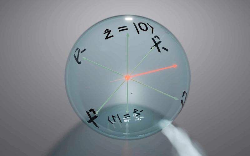
A classical bit is definitively in state \( 0 \) or \( 1 \). A quantum bit, or qubit , exists in a superposition of these states. Its state \( |\psi\rangle \) is described by a vector in a 2-dimensional complex Hilbert space:
\(|\psi\rangle = \alpha |0\rangle + \beta |1\rangle\)
where:
* \( |0\rangle = \begin{bmatrix} 1 \\ 0 \end{bmatrix} \) and \( |1\rangle = \begin{bmatrix} 0 \\ 1 \end{bmatrix} \) are the computational basis states .
* \( \alpha \) and \( \beta \) are complex numbers called probability amplitudes .
* The probability of measuring the qubit as \( 0 \) is \( |\alpha|^2 \), and as \( 1 \) is \( |\beta|^2 \). Since probabilities must sum to 1, we have the normalization condition :
\(|\alpha|^2 + |\beta|^2 = 1\)
This linear combination, \( \alpha |0\rangle + \beta |1\rangle \), is the core of quantum parallelism. A single qubit can be in a state that is both \( |0\rangle \) and \( |1\rangle \) simultaneously.
- The Nature of Quantum Gates
A quantum gate is the quantum analogue of a classical logic gate. However, there are critical differences dictated by the laws of quantum mechanics.
- *Reversibility & Unitarity: All quantum gates (except measurement) are reversible . This is mathematically encoded by the property of being a unitary transformation . A matrix \( U \) is unitary if:
\(U^\dagger U = U U^\dagger = I\)
where \( U^\dagger \) is the conjugate transpose of \( U \). Unitarity guarantees that the transformation preserves the norm (length) of the state vector, which is essential for preserving total probability.
- Action on Superposition: Because quantum gates are linear operators, their effect on a superposition state is defined by their effect on each basis state.
If \( U|0\rangle = |\phi_0\rangle \) and \( U|1\rangle = |\phi_1\rangle \), then
\(U(\alpha |0\rangle + \beta |1\rangle) \)= \(\alpha |\phi_0\rangle + \beta |\phi_1\rangle\)
This linearity is what allows quantum gates to process all components of a superposition simultaneously.
- The Pauli Gates (X, Y, Z)
These are the most fundamental single-qubit gates.
Pauli-X Gate (The Bit-Flip Gate)
\(X \)= \(\begin{bmatrix} 0 & 1 \\ 1 & 0 \end{bmatrix} \)
* Action: It flips the computational basis states.
\(X|0\rangle = |1\rangle \quad \text{and} \quad X|1\rangle = |0\rangle\)
* Analogue: It is the quantum version of the classical NOT gate.
* Effect on Superposition: For a general state, \( X(\alpha |0\rangle + \beta |1\rangle) = \beta |0\rangle + \alpha |1\rangle \). It swaps the amplitudes of \( |0\rangle \) and \( |1\rangle \).
Pauli-Z Gate (The Phase-Flip Gate)
\(Z \)= \( \begin{bmatrix} 1 & 0 \\ 0 & -1 \end{bmatrix} \)
* Action: It leaves \( |0\rangle \) unchanged but flips the sign of \( |1\rangle \).
\(Z|0\rangle = |0\rangle \quad \text{and} \quad Z|1\rangle = -|1\rangle\)
* Effect on Superposition: \( Z(\alpha |0\rangle + \beta |1\rangle) = \alpha |0\rangle - \beta |1\rangle \). This introduces a relative phase of \( -1 \) between the two basis states. The global phase is unobservable, but this *relative* phase has profound consequences.
Pauli-Y Gate
\[
Y = \begin{bmatrix} 0 & -i \\ i & 0 \end{bmatrix} = iXZ
\]
* Action: It performs both a bit-flip and a phase-flip.
\[
\begin{aligned}
Y|0\rangle &= i|1\rangle \\
Y|1\rangle &= -i|0\rangle\\
\end{aligned}
\]
This gives the formatted output:
\[
\begin{aligned}
Y|0\rangle &= i|1\rangle \\
Y|1\rangle &= -i|0\rangle\\
\end{aligned}
\]
These are the correct transformations for the Pauli Y gate, which applies a bit flip and phase flip with imaginary coefficients. The matrix representation is:
\[
Y = \begin{bmatrix} 0 & -i \\ i & 0 \end{bmatrix}
\]
- The Hadamard Gate (The Superposition Gate)
The Hadamard gate is crucial for creating superpositions from basis states.
The Hadamard gate matrix representation:
\[
H = \frac{1}{\sqrt{2}} \begin{bmatrix} 1 & 1 \\ 1 & -1 \end{bmatrix}
\]
* Action: The Hadamard gate operation on computational basis states:
\[
\begin{aligned}
H|0\rangle &= \frac{|0\rangle + |1\rangle}{\sqrt{2}} = |+\rangle \\
H|1\rangle &= \frac{|0\rangle - |1\rangle}{\sqrt{2}} = |-\rangle
\end{aligned}
\]
* The states \( |+\rangle \) and \( |-\rangle \) are known as the Hadamard basis or diagonal basis . A qubit in this state has an exactly 50% chance of being measured as \( |0\rangle \) or \( |1\rangle \).
* Key Property: \( H \) is its own inverse: \( H^\dagger H = H^2 = I \). Applying it twice returns the original state: \( H|+\rangle = |0\rangle \) and \( H|-\rangle = |1\rangle \).
- Phase Gates (S and T)
These gates introduce complex phases.
S Gate (or \( \frac{\pi}{2} \)-Phase Gate)
\(S \)= \(\begin{bmatrix} 1 & 0 \\ 0 & i \end{bmatrix}\)
* Action: \( S|0\rangle = |0\rangle \) and \( S|1\rangle = i|1\rangle \). It is the square root of the Z gate: \( S^2 = Z \).
T Gate (or \( \frac{\pi}{4} \)-Phase Gate)
\(T\) = \(\begin{bmatrix} 1 & 0 \\ 0 & e^{i\pi/4} \end{bmatrix}\)
* Action: It is the square root of the S gate: \( T^2 = S \). This gate is essential for achieving universal quantum computation.
- Multi-Qubit Gates: Entanglement
Quantum computation's true power emerges with multi-qubit gates, which can create entanglement -a strong correlation between qubits that cannot be replicated classically.
CNOT Gate (Controlled-NOT)
This is the fundamental 2-qubit gate.
\(\text{CNOT}\) = \(\begin{bmatrix} 1 & 0 & 0 & 0 \\ 0 & 1 & 0 & 0 \\ 0 & 0 & 0 & 1 \\ 0 & 0 & 1 & 0 \end{bmatrix}\)
* Action: It has a control qubit and a target qubit.
* If the control is \( |0\rangle \), it does nothing.
* If the control is \( |1\rangle \), it applies an X gate to the target.
\[
\begin{aligned}
\text{CNOT}|00\rangle &= |00\rangle, \\
\text{CNOT}|01\rangle &= |01\rangle, \\
\text{CNOT}|10\rangle &= |11\rangle, \\
\text{CNOT}|11\rangle &= |10\rangle
\end{aligned}
\]
In summary: \( \text{CNOT}|c, t\rangle = |c, t \oplus c\rangle \), where \( \oplus \) denotes addition modulo 2 (XOR).
* Creating Entanglement: The CNOT gate, combined with the Hadamard gate, can create a Bell state , a maximally entangled state.
\( \text{CNOT} \cdot (H \otimes I) |00\rangle = \text{CNOT} \left( \frac{|0\rangle + |1\rangle}{\sqrt{2}} \otimes |0\rangle \right) = \frac{|00\rangle + |11\rangle}{\sqrt{2}} = |\Phi^+\rangle \)
In this state \( |\Phi^+\rangle \), the measurement outcomes of the two qubits are perfectly correlated. Measuring one qubit instantly determines the state of the other, regardless of the distance between them.
- Applying Gates to Multi-Qubit Systems
When dealing with \( n \)-qubit systems, the state is a vector in a \( 2^n \)-dimensional space. To apply a single-qubit gate to a specific qubit in a multi-qubit system, we use the tensor product with the identity matrix \( I \) on the other qubits.
* Example: Applying an \( X \) gate to qubit 1 in a 2-qubit system is represented by \( X \otimes I \).
\((X \otimes I) |00\rangle = (X|0\rangle) \otimes (I|0\rangle) = |1\rangle \otimes |0\rangle = |10\rangle \)
* Index Notation: \( X_1 |00\rangle = |10\rangle \) is a common shorthand, meaning "apply X to the qubit at index 1."
This foundation in how quantum gates manipulate superposition and create entanglement is the absolute prerequisite for tackling advanced topics like quantum algorithms and, as in your assignment, quantum error correction , where gates like X and Z are used to detect and correct for "bit-flip" and "phase-flip" errors without collapsing the delicate quantum data.