A Deep Dive into Classical Activation Functions Derivation, Properties, and Use Cases
Introduction
Activation functions are the cornerstone of artificial neural networks. They introduce non-linearities into the network, allowing it to learn and model complex, real-world data patterns beyond simple linear regression. Without them, a multi-layer neural network would simply collapse into a single linear layer. This article explores the foundational, classical activation functions, providing a step-by-step mathematical derivation of their gradients and a clear analysis of their advantages, disadvantages, and modern use cases.
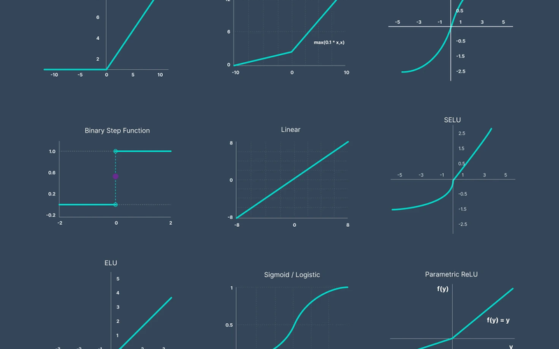
- Step Function (Heaviside Function)
The Step Function was used in the very first computational model of a neuron, the McCulloch-Pitts neuron, and in the original perceptron.
Formula:
\[ f(x) = \begin{cases} 0 & x < 0 \\ 1 & x \geq 0 \end{cases} \]
Range: {0, 1}
Derivation of the Gradient
The derivative of a function at a point gives us the slope or the rate of change at that point.
* For \( x < 0 \), the function is a constant value of 0. The derivative of a constant is 0 .
* For \( x > 0 \), the function is a constant value of 1. The derivative of a constant is 0 .
* At \( x = 0 \), the function is discontinuous. The derivative is technically undefined (infinite slope).
Derivative:
\[ f'(x) = \begin{cases} \text{Undefined} & x = 0 \\ 0 & x \neq 0 \end{cases} \]
In practice, the derivative at \( x = 0 \) is treated as 0 to avoid computational issues, but the fundamental problem remains.
Analysis in Point Form
* Advantages:
* Simple & Interpretable: Mimics the "all-or-nothing" firing of a biological neuron. The output is a clear binary signal (ON/OFF).
* Theoretical Foundation: Crucial for the historical development of neural network theory.
* Disadvantages:
* Non-Differentiable: The discontinuity at \( x=0 \) means it has no defined gradient at that point. This makes it incompatible with gradient-based optimization methods like Backpropagation, which require a derivative to update weights.
* Vanishing Gradients: For all \( x \neq 0 \), the gradient is exactly 0. This means that during backpropagation, no weight updates will occur, and learning will stop completely. This is the most severe form of the "vanishing gradient" problem.
* Binary Output: It cannot model intermediate values, making it useless for multi-value classification or regression.
* Modern Use Case:
* None in Deep Learning. It is obsolete for training modern neural networks due to its non-differentiability. Its primary use is now in historical context and theoretical explanations.
- Linear (Identity) Activation Function
The Linear activation function simply returns its input without any transformation.
Formula:
\[ f(x) = x \]
Range: (-∞, ∞)
Derivation of the Gradient
The derivative is straightforward, as it is a linear function with a slope of 1.
Derivative:
\[ f'(x) = 1 \]
Analysis in Point Form
* Advantages:
* Prevents Vanishing Gradients: The gradient is always 1, ensuring that gradients flow backwards through the network without diminishing.
* Simple and Computationally Efficient.
* Disadvantages:
* No Non-Linearity: This is the most critical flaw. A deep network of multiple linear layers is equivalent to a single linear layer. i.e., \( W_3(W_2(W_1x)) \) can be collapsed into a single operation \( W_{final}x \). This defeats the entire purpose of having a deep network, which is to learn hierarchical, non-linear features.
* Unbounded Output: The output is not constrained, which can be unstable in multi-layer networks and makes it unsuitable for predicting probabilities (which must be between 0 and 1).
* Modern Use Case:
* Output Layer for Regression Tasks: It is commonly used in the output layer of a network designed to predict a continuous value (e.g., predicting house prices, temperature, or a quantity). Here, we want the network's output to be able to take on any real number.
- Sign Function
The Sign Function is similar to the Step Function but outputs -1 or +1 instead of 0 or 1.
Formula:
\[ f(x) = \text{sign}(x) = \begin{cases} -1 & x < 0 \\ 0 & x = 0 \\ 1 & x > 0 \end{cases} \]
Range: {-1, 0, 1} or more commonly {-1, 1} in practice.
Derivation of the Gradient
The derivative follows the same logic as the Step Function.
* For \( x < 0 \), the function is a constant value of -1. The derivative is 0 .
* For \( x > 0 \), the function is a constant value of 1. The derivative is 0 .
* At \( x = 0 \), the function is discontinuous and the derivative is undefined .
Derivative:
\[ f'(x) = \begin{cases} \text{Undefined} & x = 0 \\ 0 & x \neq 0 \end{cases} \]
Analysis in Point Form
* Advantages:
* Binary Output with Zero Center: Outputs -1 and +1, which can be beneficial as it produces zero-centered data, unlike the Step Function. This can sometimes help during the learning process.
* Disadvantages:
* Non-Differentiable: Shares the same fundamental flaw as the Step Function. It has no usable gradient for learning and is incompatible with backpropagation.
* Vanishing Gradients: The gradient is zero almost everywhere, halting learning.
* Modern Use Case:
* None in Deep Learning Training. Like the Step Function, it is obsolete for training.
* Theoretical Models & Binarized Neural Networks (BNNs): It finds a niche in advanced research areas like BNNs, where weights and activations are constrained to +1 or -1 (or 0/1) for extreme computational efficiency on specialized hardware. However, even in BNNs, a "Straight-Through Estimator" (STE) is used during training to approximate the gradient, as the true derivative is zero.
Summary
Step Function
* Formula: \( f(x) = \begin{cases} 0 & x < 0 \\ 1 & x \geq 0 \end{cases} \)
* Range: {0, 1}
* Derivative: 0 everywhere, and undefined at x=0.
* Primary Advantage: Its output is very simple and interpretable (on/off).
* Fatal Flaw: It is non-differentiable and has a zero gradient, making it impossible to use with gradient-based learning.
* Modern Use Case: None; it is only of historical interest.
Linear Function
* Formula: \( f(x) = x \)
* Range: (-∞, ∞)
* Derivative: 1
* Primary Advantage: It completely avoids the vanishing gradient problem.
* Fatal Flaw: It is not a non-linear function, so a network of only linear layers can only learn linear relationships.
* Modern Use Case: Typically found in the output layer for regression tasks.
Sign Function
* Formula: \( f(x) = \text{sign}(x) \) (Outputs -1 if x<0, +1 if x≥0)
* Range: {-1, 1}
* Derivative: 0 everywhere, and undefined at x=0.
* Primary Advantage: Its output is zero-centered (-1 and +1).
* Fatal Flaw: It is non-differentiable and has a zero gradient, similar to the step function.
* Modern Use Case: Specialized research areas, such as in Binarized Neural Networks.
Conclusion
The classical activation functions, while foundational, reveal the core challenges that led to the development of modern deep learning. The Step and Sign functions demonstrated the absolute necessity of differentiability for gradient-based learning. The Linear function highlighted the critical need for non-linearity to unlock the representational power of deep networks.
The shortcomings of these classical functions directly motivated the creation of the "modern classics" like the Sigmoid , Tanh , and ReLU families, which are designed to be non-linear, differentiable, and to permit better gradient flow, enabling the training of the deep, powerful neural networks we use today. Understanding these early functions is key to appreciating the evolution and core principles of neural network design.


